This lab will further your skills on vector analysis by computing the restoration funds that might be available for Humboldt County Forests.
We'll also be reviewing:
To setup for this assignment:
1. Create a folder structure on "D:" as we have done before:
2. Download the data into the "Originals" folder, unzip it, and make sure the spatial references are defined correctly.
3. The spatial reference system for this lab is "North American Datum 1983, Universal Transverse Mercator Zone 10 North" or "NAD 83, UTM Zone 10 North". Copy data sets that are in this spatial reference from the "Originals" folder to the "Working" folder and "Project" any data sets that are not in this spatial reference to the "Working" folder.
Note: Data using the State Plane Coordinate System can be in either feet or meters. Be sure you read the metadata very carefully to determine whether feet or meters are the linear unit associated with any data using the State Plane Coordinate System.
Note: If you project a layer from one coordinate system to another and you see an error message that states "A locator with this name does not exist. Failed to execute (Project)", this may indicate that the coordinate system of that layer was incorrectly defined prior to using the project tool (e.g., it was defined as State Plane "Meters", when it was actually in State Plane "Feet").
As you begin working on more and more complex analysis tasks, you'll want to be able to diagram the steps you'll be using both for your own reference and to share with others. Microsoft PowerPoint is very easy to use to create flow charts.
1. Open PowerPoint.
2. From the "Home" tab, select "Layout" and then the "Blank" layout.
3. In the "Drawing" panel of the "Home" tab, you'll either see a drop down menu for "Shapes" or a palette of shapes with a drop down in the corner. Click on the drop down and you should see a large "palette" of shapes to select from.
 or
or 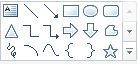
Tool bar options to access shapes
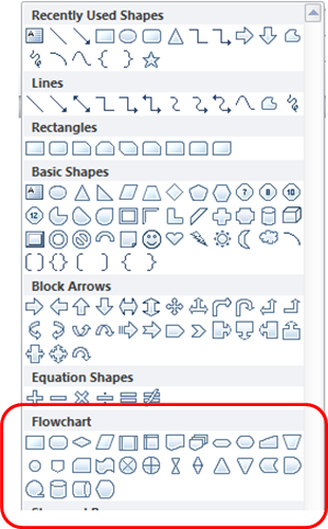
Shape Palette
There are a large number of flowchart shapes available but we'll only be using:
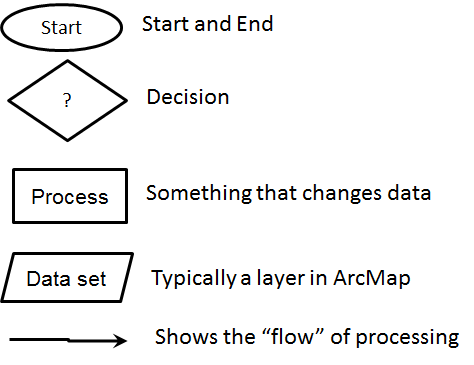
Basic Flow Chart Symbols
4. To get started, click on the oval shape and then press down and drag in the area of the slide.
5. Right-click in the shape and select "Edit Text".
6. You should see a blinking "caret" appear. Type the word "Start".
7. Now repeat with a rectangle for a "Process" block.
8. From the "Lines" section of the shape palette, select the "Elbow Arrow Connector". This is a special connector that will move with shapes once it is connected to them.
9. Move your mouse near the edge of a shape and you should see little boxes appear. Press your mouse in one of these boxes and then drag to the edge of another shape. You should see more little boxes appear on the other shape. Release the mouse button while in one of these boxes.
10. Now, drag the shapes around and you'll see that they are connected.
11. Continue with this until you have a flow chart with at least a "Start" shape, an "End" shape, a couple of process shapes, a couple of data set shapes, and lines connecting all of them.
12. Decision shapes are special shapes to determine the "direction" your processing will take. Let's say that you had a large number of raster files to process and you only wanted to process those that did not contain clouds over HSU. You might use the flow chart below.
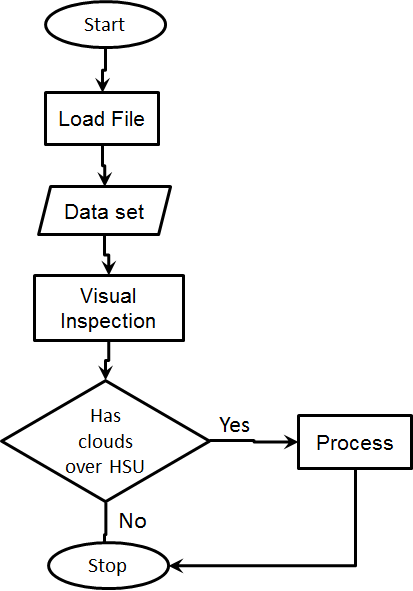
Note that the flow chart above has symbols for "Load File" and "Data set". These will not always be needed. The level of detail you provide in the flow charts is up to you but typically folks put in too little to start so if you're not sure whether to include a step, include it.
Model Builder in ArcMap uses different symbology than those presented above. Below is a flow chart created in PowerPoint using the symbols that are similar to the ones in Model Builder. You can use this as a started point for your flow chats instead.
These are the "standard" symbols but there are a lot of variations on the standard. Any symbology that works and has a legend is appropriate.
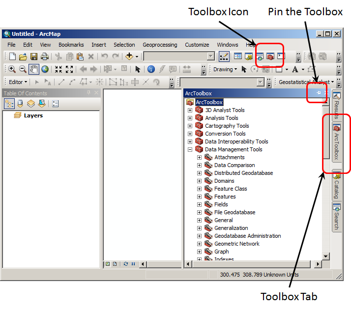
The ArcToolbox contains a huge number of tools for spatial analysis and processing. You can open the tool box by clicking on the "Toolbox Icon". Then, you'll probably want to click on the little icon of a "pin" to "Pin the Toolbox" to the side of ArcMap if a tab for "ArcToolbox" does not already appear.
It can also be a little hard to find what you are looking for. Take some time now to get to know where things are in the toolbox. Some of the make "toolboxes" you'll use are:
It can be challenging to find the right tool for a job in the ArcToolbox. You may need to use the Web to find the name by typing "<something about the tool> ArcMap" into a search engine and then you should find the tool that ArcToolbox uses (such as "Dissolve" for performing a union within a layer). Once you know the name, you can enter it into a search and the name of the tool will appear. Then, you can click on the name to access the tool.
You'll want to make a "notebook" for the tools you use, their names, and where to find them so you can get back to them quickly.
1. Go to the ArcGIS Toolbox and open the "Analysis Tools" toolbox.
2. Open the "Proximity" "toolset" (toolsets are inside a toolbox) and you'll see "Buffer".
3. Double-click on "Buffer" and you'll see this is exactly the same tool that is under the "Geoprocessing" menu.
4. Close the "Buffer" tool without running it and open the "Search" tab and enter "Buffer".
5. Click on "Buffer(Analysis)" and you'll again see the "Buffer" tool.
There are many ways to access tools in ArcMap. How you find them is up to you but we still recommend at least writing down the name of the tools you use so you can find them with "Search".
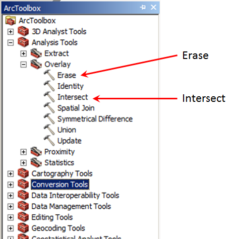
For this lab, you'll need to use the tools we've examined before and the "Erase" and "Intersect" tools. They can be found in the "Overlay" toolset.
Below is a hypothetical problem in spatial analysis. Pretend that you are a GIS analyst with the US Forest Service and you've been asked to create a short report explaining the potential impact of the situation below.
Problem
Congress is proposing an allocation of stream restoration dollars to U.S. Forest Service lands. The amount of money to be allocated to each National Forest will be based on three factors:
It is your job to conduct a spatial analysis to determine what these values are, so that congress will know how much money to allocate to each National Forest for stream restoration efforts.
1. Find the total length of streams in each National Forest jurisdiction
This section will rely upon skills you've learned before and performing "Joins and Relates".
1. Create a layer that only contains the polygons that are under National Forest Service jurisdiction. This can be found in the AGENCY_NM field of the Humboldt Ownership layer.
2. Then, clip the streams layer to just the National Forest lands. You do not need to specify an "X,Y Tolerance" when you run your overlay operation.
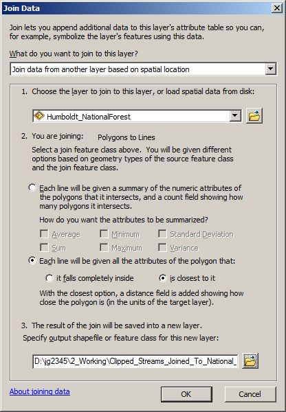
3. Now we need to connect the streams to the forest they reside in. We can do this with a "Spatial Join". Right click on the your clipped streams layer and select "Joins and Relates -> Join...".
4. Select your layer that contains the National Forests for item "1.", "the layer to join to".
5. Select "Each line will be given all the attributes of the polygon that:" for item "2. You are joining" and select "is closest to it". This is an important step because ArcMap will not include polylines if there are any misalignments at the edges of the forest boundaries.
6. Give the new layer an appropriate name and the dialog should appear something like the one below:
7. When the join is completed, open the attribute table for the new layer and you should see the attributes, including the "AGENCY_NM" field have been added to the features.
8. Add a new field for a "Length" or update the existing one with the length of each stream feature in meters.
9. ArcMap has the ability to "Summarize" statistics based on common attributes between features. Right-click on the field with the agency name ("AGENCY_NM") and select "Summarize". We want to find the "Sum" of all the lengths of streams by agency so select the "Sum" of your length field as item 2, the "statistic to be included in the output table.
10. ArcMap will ask you if you want to add the table and you'll want to say "Yes".
11. Now, right click on the new table and select "Open" to see the total (sum) of the lengths of stream in the forests broken up by agency.
12. We want to include the lengths in our final report but it is difficult to make professional looking tables in ArcMap. You can "Export" data from any table by opening the table, clicking on the icon in the upper left, and selecting "Export...". Then, you can export the data to a "Text file" that you can open in Excel. Since this is a very small table, we can simply insert a table into MS-Word and copy and paste the values from ArcMap into the table. To add a table to MS-Word, select the "Insert" tab and then press and drag to create a new table. When you release the mouse button, the table will be added to your document. Then, you can just type values into the table.
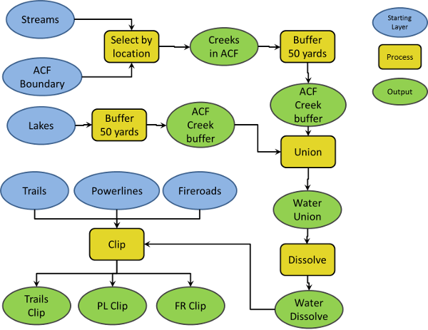
13. Below is an example flow chart and there is also a PowerPoint version of the flow chart that you can use to help you create the additional charts for this lab. Note that this flow chart is slightly different than the current approach described in this lab.
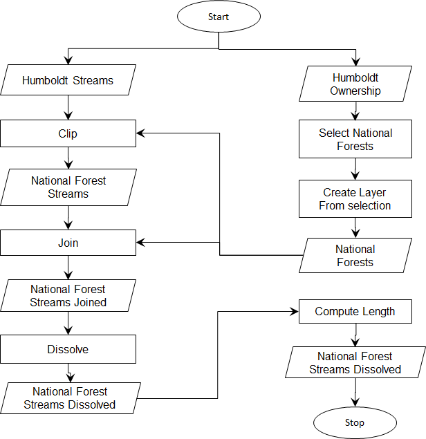
Note: While you can use this flow chart as the first one in your report, you must always cite the source of any material you use. You'll need to create new flow charts for each of the following sections but if you use parts of the one above, you need to cite them appropriately (i.e. "Adapted from the HSU GSP 270 Lab 9 materials").
2. Find the total amount of land legally available for timber harvesting in each National Forest jurisdiction.
Now that you have determined the total length of streams in each National Forest jurisdiction, your second task will be to determine the total amount of harvestable land in each National Forest. Timber harvesting regulations prohibit timber harvesting practices within a given distance of streams. For this exercise, we will say that the legal distance is based on the stream class. Timber harvesting may not occur within a distance of 250 meters from a type 3 stream, within 200 meters of a type 2 stream, or within 100 meters of a type 1 stream. So, to find the answer to Part 2, you will first need to create a variable distance buffer around the streams in the National Forests (i.e., around the streams you created in the previous section). This buffer zone will define areas in which timber harvesting is prohibited (which we can then use to identify areas in each National Forest where timber harvesting is legal).
1. Return to your clipped National Forest streams layer and add a field for the distance to buffer each stream type called something like "buff_dist". Calculate the values in that field based on the stream TYPE.
Note: This step can be completed by switching back and forth between "Select by Attributes" and "Field Calculator". First, use "Select by Attributes" to select the "TYPE 3" streams, then use field calculator to set the selected streams to 250. You can do this by just entering "250" in the equation area. Then, repeat this for the other types.
2. Now we need to find the areas around the streams not available for timber harvesting. Open the "Buffer" tool and buffer the streams using the "buff_dist" field created earlier.
3. Set the "Dissolve Type" to "LIST" and then put a check next to "AGENCY_NM" in the "Dissolve Fields(s)" list. This will ensure that the output will maintain information about which National Forest each stream buffer is associated with.
Important: This is a variable distance buffer, so do not use the option to buffer by a "linear unit", otherwise all streams would get buffered by the same distance. You could accomplish this same task by breaking the layer into one data set for each of the stream types and then merging them back together but this approach will make it easy to handle data sets with many different attribute values.
Question 1: Where will the units come from for the variable distance buffer since we did not specify it?
4. Find the portions of land within each National Forest that are outside of the buffered areas you just created and which may, therefore, be legally harvested for timber (again, do not set an x,y tolerance when running your overlay operation). You will have to determine which overlay operation that we have discussed will allow you to accomplish this. You can search for "overlay toolset" in the ArcGIS help files to get additional help with this.
5. Now you just need to create an "Area" field in the attribute table, summarize the area as we did in the previous exercise, and add a table with the results to MS-Word.
Note: Remember to update the area field for the features in your new layer (specify square meters as the units).
3. Find the total length of class 40 roads in the streams buffer for each National Forest.
For the final component of this analysis you will need to determine the total length in meters of class 40 roads (that is, roads where Class = 40) within the streams buffer you created in Part 2 for each National Forest Jurisdiction. Class 40 roads are main roads that are paved. Note that some of the buffer zones you created in Part 2 fall outside the National Forest boundaries (Zoom in and investigate). However, if part of a road is within this buffer zone, it is still within the specified buffer distance of a stream within the National Forest. Therefore, it needs to be included in this calculation.
The attribute table of the streams buffer will indicate which National Forest each buffer zone is associated with. Therefore, the only two layers which you will need to use in order to find the answer are the Roads Layer and the Streams Buffer layer.
The total dollar amount to be allocated to each National Forest is determined by the following formula:
$ Amount Allocated = .3(stream length) + .1(area) + .2(road length)
You can use excel, a calculator, the windows calculator, Google, or anything else that does math to make your calculations.
A short report that includes your results from Exercise 1.
Note: The area of interest is rather long from north to south making it challenging to create a small map. I would recommend putting Humboldt county behind the map and then making the map almost full-page size so the detail is visible.
Note: Make sure all the text in your maps is readable and above 9 point. You do not need to include your name or the data in the map as your name and the date will be on the overall document. You can also move the information on spatial reference and data sources to the caption to simplify the map. Also remember to define all acronyms before using them and spell check your document before turning it in. We will begin deducting more points if these items are not addressed in this and future labs.
© Copyright 2018 HSU - All rights reserved.