Lab 7: Research Sites, Part 2 - Creating Streams and Watersheds

Introduction

In the previous lab, we learned where to acquire data and how to perform a standardized quality assurance and quality control procedure. Now that we have the data, we will prepare it for analysis by projecting the data into the same projection and coordinate system. Once this is done, we will create some additional data sets and run some basic calculations.

The key questions we are trying to ask with this lab are:

1. How many streams are there in Arcata Forest and what is their total length?
2. What are the watersheds in Arcata Forestry and how large are they?

Learning Outcomes

• Use the " Project " tool to project data into the same spatial reference
• Create stream networks and watersheds from a DEM
• Use Raster Calculator for simple raster math.
• Create fields (attributes) and compute length and area.
• Create maps that convey results of spatial analysis

Clipping The Wetlands Data

One of the layers we want to look at are the wetlands for California but the data set is huge! If you have not done so already, "clip" it to just Humboldt County. In ArcGIS:

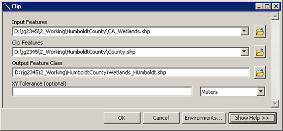
1. From the "Geoprocessing" menu, select "Clip"
2. For the "Input Features" use the "CA_Wetlands" shapefile (depending on the downloaded file, it may be "CA_Wetlands_North").
3. For the "Clip Features" use the Humboldt County Boundary.
4. Set the "Output Feature Class" to "Humboldt_WetLands.shp" and save it in the "Humboldt_County" "Working" folder.
5. When you click "OK", ArcMap will take a few minutes and then should display a wetlands shapefile for just Humboldt County that will load and redraw much faster than the one for all of California.

 

Walk Through: Projecting Vector Data

It is important that each layer in any analysis you perform have the same spatial reference system. This will minimize uncertainty and error. Any error related to map projections will at least be uniform throughout the analysis if they all share the same spatial reference system.

In this step we will project each of our data sets into WGS84 UTM Zone 10 North. This is an international coordinate system based on the Transverse Mercator projection. It is particularly accurate for regions with a North/South orientation, such as Humboldt County. UTM always uses meters as the linear unit.

1. Using the folder structure from the last lab, download the Arcata Forest data and add it to your "1_Originals" folder. I have checked these data sets and they are all in "WGS_1984_StatePlane_California_I_FIPS_0401_Feet" and appear OK except that some of them cover a larger area than just the forest.
2. Also, download the results from our digitizing lab and unzip the file.
3. Create a "2_Working" folder next to your "1_Originals" folder.
4. Launch ArcMap and open a blank map document (.mxd).
5. Navigate to "Data Management Tools -> Projections and Transformations", and select the "Project" tool.
6. Select the "CA_Wetlands" data set for the "Input Dataset"
7. Save the output data set to your "2_Working" folder and give it a good name such as "Humbolt_County_Wetlands.shp"
8. Make sure to set the "Output Coordinate System" to WGS 84, UTM Zone 10 North
9. Repeat this process for the following data sets:
   1. apnhum53sp.shp -> Humboldt_Parcels.shp
   2. humtrans3sp_20130417.shp -> Humboldt_Roads.shp
   3. From the Arcata Forest data set:
      1. cfroads83v7 -> Forest_Roads.shp
      2. creeksp83v13 -> Forest_Creeks.shp
      3. cftrails83v8.shp -> Forest_Trails.shp (I believe this is "version 8" but I did not see any differences between this an "v7")
      4. ACF_boundarysp83v3.shp -> Forest_Boundary.shp
      5. waterbodysp83v10.shp -> Forest_Waterbodies.shp
   4. "Streams" from lab week's lab -> Class_Streams.shp

Once the project tool is complete, you should see a copy of each of these layers in your "2_Working" folder.

Walk Through: Projecting Raster Data

Now that we have our shapefiles in the correct projection, we will do the same for our raster data. You will find that most tools require a separate set for raster and vector data. In this case we will use the "Project Raster" tool.

1. Navigate to "Data Management Tools", "Projections and Transformations","Raster", and select the "Project Raster" tool.
2. From the data you downloaded last week, select the DEM "imgn41w125_13.img" for the "Input Raster"
3. For the "Output Raster Dataset" be sure to save to your working folder. Call the output "WestDEM.img". The "img" or "Imagine" file format is the best file format for rasters when working with ArcGIS.
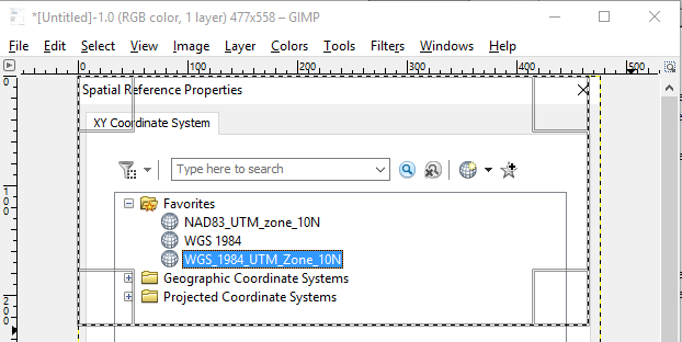
4. For the "Output Coordinate System", open the Spatial Reference Properties window by clicking the icon on the right. Just as before, we can use the "Layers" folder to select "WGS_1984_UTM_Zone_10N".
5. Make sure to change the "Resampling technique" to "Bilinear" or you'll have really bad artifacts (vertical and horizontal lines) in your DEM. You won't see them until you run a hillshade or direction algorithm but they will be there.
6. Select "BILINEAR" for the "Resampling Technique" or you will have artifacts in your DEM that will show up when you create direction or hillshade rasters from it.
7. Leave the remaining default settings as they are and click OK.

Ready for Analysis?

When completed, you should have folders in your "2_Working" folder that contain data for Humboldt County and Arcata Forest. All the data should be in the same spatial reference and ready for us to do some Spatial Analysis!

A great thing to do before proceeding is to select "File -> New" in ArcMap and then load all your files from the "2_Working" folder into the program. You should not receive any warnings or errors. If you do, something went wrong and you'll want to fix it before proceeding.

Streams Data

Streams data is very important to natural resource research but it is also very challenging to find a "good" stream layer, especially at high resolution. In this step, we'll take a look at some existing stream layers and then create one of our own.

Comparing Water Body Layers

1. In ArcMap, load the data sets for:
   1. Arcata Forest Boundary
   2. Arcata Forest Creeks
   3. Streams from the last lab
   4. California Wetlands that were clipped to Humboldt County
2. Zoom in to the layers and take a minute to examine the layers.

Clipping Rasters to an Area

The bottom line is that none of the water body layers we have are going to work for the research we want to do in Arcata Forest. Because of this, we need to create a new stream layer. I recommend walking through these steps rather carefully as a wrong turn can cause your computer to crash or take a really long time to finish processing.

First, to make the stream network processes move fast, we need to clip the DEM to just the area around Arcata Forest.

1. If the "Draw" tool bar is not visible, right click in the blank area of the menu bar in the top-right area of ArcMap and select "Draw".
2. Draw a "box" around Arcata Forest with plenty of room on the sides. The box should be about four times as large as the forest.
3. In the "Draw" toolbar, select "Convert Graphics To Features" in the "Drawing" menu. This feature allows us to convert a drawn element into a feature in a shapefile which is really handy.
4. Set the "Output shapefile" to be a file called "ClippingBoundary.shp" and store it in your "Arcata Forest" folder in your working folder.
5. When you click "OK" you'll see the boundary added as a layer.
6. Click on the original box you drew and then click the "Delete" key on the keyboard. This will delete the box you draw but the feature in the shapefile should still be visible.
7. Clipping rasters is different from clipping vectors so open the search box and type in "Clip Raster"
8. The first item should be "Clip" in "Data Management". Select this tool.
9. Select the DEM as the "Input Raster" and the "ClippingBoundary" as the "Output Extent". Then, set the "Output Raster" to "DEM_Clipped.img" in your Arcata Forest working folder.
10. The clipped DEM should appear around your Arcata Forest boundary.

Checking for Artifacts and Creating Hillshades

Before continuing, we want to make sure our DEM does not have any artifacts that could cause problems (this happens a lot with DEMs). A handy tool for this, and making backgrounds on maps is the "Hillshade" tool.

1. In the ArcToolbox, navigate to "Spatial Analyst -> Surface -> Hillshade". If you receive an error that you do not have a license for these tools, go to "Customize -> Extensions" and select "Spatial Analyst".
2. Select our clipped DEM for the "input raster"
3. Give the "Output raster" a good name like "Hillshade.img" and save it in the Arcata Forest working folder.
4. For now, we'll leave the "Azimuth" and "Altitude" values at the defaults as these are also the default for most western maps.
5. When you click "OK", you should see a simulation of light reflecting from the topography as if the sun were to the north west. If you see any lines running through the hillshade that should not be there then you have "artifacts" in the image from processing or the original data collection and you'll run into problems down the road.
6. Hillshades are very commonly used for backgrounds on maps as well. As long as we're here, let's make on.
7. Right click on your DEM and select "Properties".
8. Select the "Symbology" tab and change the "Color Ramp" to something more interesting.
9. Right click on your Hillshade layer and set the "Transparency" to 50%.
10. When you have a chance, come back to these steps and play with the color ramps and other settings to make nice backgrounds for this report and future ones.
11. Note: Change the "Brightness" in the "Display" tab of both rasters to make the hillshade fade into the background.

Creating a Stream Network

Creating a stream network requires a number of steps but should work out if you are careful (or are ready to go through the process several times).

1. Load the DEM that is clipped around Arcata Forest from the previous section.
2. Open the "ArcToolbox" and "Spatial Analyst Tools" -> Hydrology". If you receive an error that you do not have a license for these tools, go to "Customize -> Extensions" and select "Spatial Analyst".
3. Before we work with a DEM we have to "Fill" any "Holes" in the DEM. These are pixels that have very low values and will cause a stream to disappear during processing (take a look at your existing streams layers and see if you can find the one that was done with a DEM without the holes filled). Select the "Fill" tool.
4. Select our clipped DEM for the "Input surface raster"
5. Name the "Output surface raster" "Filled.img" and save it into the Arcata Forest working folder. When you click OK, you should see a new DEM that looks just like the old one.
6. The next step is to create a raster that shows the direction that water will flow downhill. Select the "Flow Direction" tool.
7. Use our filled DEM for the "Input surface raster"
8. Set the "Output flow direction raster" to "Direction.img" and save it into the Arcata Forest working folder. you should see a very brightly colored image where the pixels have been given "codes" for the cardinal direction (N, NW, W, SW, S, etc.) for the direction that water would flow from this pixel.
9. We'll now use the Direction raster to create a raster where each pixel represent the number of pixels that "flow" or "accumulate" into it. Select the "Flow Accumulation" tool.
10. Select the "Direction" raster for the "Input flow direction raster" and give the output raster a name like "Accumulation.img" and save it in the "Arcata Forest" working folder.
11. After you click "OK", you should see a few lines that are the ends of the streams that appear in the DEM. To see these better, right click on the "Accumulation" layer and select "Properties".
12. Click on the "Symbology" tab and make sure "Show" is set to "Stretched".
13. Change the "Color Ramp" to something more interesting and set the "Type" to "Standard Deviations". This should make it easier to see the streams.
14. Next, we need to create a raster that contains 1's where we want the steams to be and 0's elsewhere. In the ArcToolbox, navigate to "Spatial Analyst -> Map Algebra" and open the "Raster Calculator". This is a powerful tool that lets you do mathematical and other operations on entire rasters. Double click no the "Accumulation" raster and then type ">100".
15. Name the output file "Accumulation_GreaterThan_100.img".
16. 
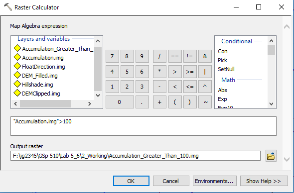
17. When you click "OK", you should see a raster with 1's where the pixels along the streams have "accumulated" the water from over 100 other pixels.
18. Try one at 1000 pixels and some other values. Note that this tool is handy for making streams at different levels of detail for research and for cartography.
19. Our last step is to convert these rasters to polylines that represent a stream network. Open the "Search" tool and enter "Raster to Polyline".
20. Use your Accumulation_GreaterThan_100" raster for the "Input rater" and name the output "Streams_Over_100.shp".

Clean up

You may have noticed some little squares where the conversion to polyline followed multiple paths for your streams. These are not desired so we'll need to remove them.

1. Clip the streams to just the boundary we used for clipping the DEM (i.e. a boundary larger than the forest boundary) and use the new stream shapefile for this section.
2. Open the attribute table.
3. Start and edit session.
4. Zoom in to one of the areas with the extra polylines.
5. Select some of the extra polylines.
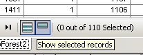
6. At the bottom of the attribute table window, select the icon to "Show selected records". This will allow you to view just the selected records and you should now see the rows for the features you selected.
7. 
8. Right click on one of the rows and select "Delete Selected".
9. The rows should disappear and the extra polylines with them.
10. Repeat this process until all the extra polylines within the forest are gone and then, stop the edit session.
11. You also may have noticed that the stream reaches are broken into far more segments than needed. Run the "Unsplit" tool to join the streams into their correct reaches.

When completed, you should have a stream network that is a visible improvement over some of the other layers and, even more critically, it matches your DEM exactly for future analysis!

Comparing Results

Load your other water body layers into ArcMap and compare them with your new stream layer. Add a map for this new layer to your report.

Finding the Watershed

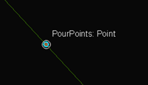
Using our direction raster we can create a polygon shapefile that describes the "watersheds" in our area of interest. First, we need to create a point file that contains "pour points". These are the points where the water will "flow" through the streams. ArcGIS uses these as a starting point and will then backtrack using our direction raster until it reaches the ridges that define our watersheds.

1. Create a point shapefile as we have done before (right click on the folder in ArcCatalog, select "New Shapefile", etc.).
2. Name the file "PourPoints.shp".
3. When you create the file, make sure to set the spatial reference to match your existing layers. A short cut is to "Import" the spatial reference from one of your existing files.
4. 
5. When digitizing your points, make sure to zoom in and the tool should "snap" to your polyline for your stream.
6. 
7. Your selection of points is also important. Try to find areas of stream reaches that are away from tributaries and low in the watershed. This will reduce the number of points you need.
8. Make sure to "Stop Editing" when you feel you have a good set of points.
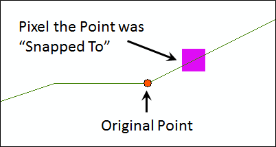
9. Before creating the watershed, we need to make sure our points are actually on the accumulation raster pixels that the stream flows through.
10. Open the "Hydrology" tool-set in Spatial Analyst and select "Snap Pour Point". This feature will create a raster with pixels that are in exactly the location we need.
11. Select your pour point shape file for the first input.
12. Select the "FID" as the "Pour point field" so we have a unique value for each pixel in the watershed.
13. Select the accumulation raster you made above for the "Input accumulation raster".
14. Give the raster a good name and save it in your working folder.
15. The "Snap distance" is how far ArcGIS should look for the highest value (our stream course) in map units (i.e. meters). Enter a value that is a few pixels across (if you've forgotten the resolution of our rasters, you can check in "Properties -> Source".
16. Zoom into one of your pour points and you should see a pixel nearby. Grab the "Info" tool and check that the pixel value matches the FID of the point nearby.
17. 
18. Finally, select the "Watershed" tool from the ArcToolbox.
19. Select our direction raster for the first input.
20. Select the "pour point" raster you just created for the second input.
21. Give the watershed output a good name and save it in the working folder.
22. When done, you should see watersheds for Arcata Forest. However, don't be surprised if this does not work the first time. You will probably have to go back to step 7 and add pour points or move them to be on top of the right accumulation pixel to catch all the watersheds.

Warning: Do not create mulitple files with pour points and then try to merge them together. The watershed tool relies upon a single set of pour points to accuracly determine the watersheds.

Arcata Forest drains into two main watersheds, the Mad River and Arcata Bay! Depending on the pour points you selected, you may see many more "watersheds" or fewer depending on where you placed your pour points.

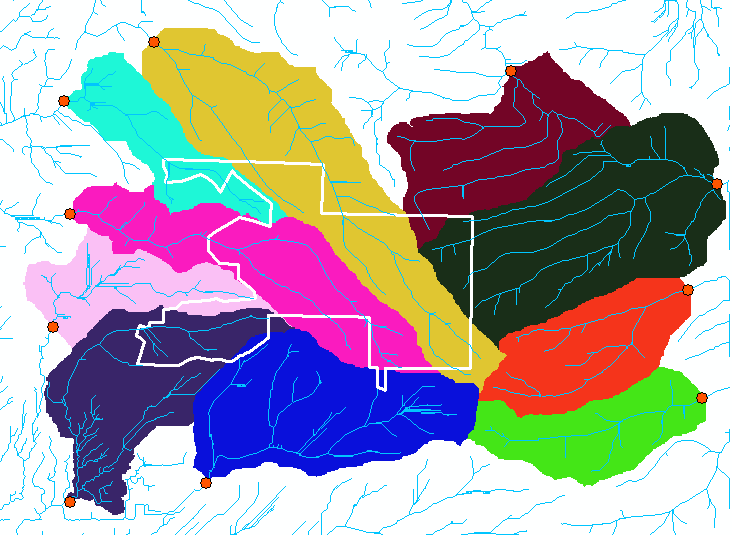
The last step is to convert this into a polygon shapefile which will be much easier to work with and will be easier on the eyes!

1. In the search box, enter "Raster to polygon".
2. At this point, we're going to be giving you fewer instructions in the labs as you're beginning to master running ArcGIS. For this tool, just make sure to uncheck the "Simplify polygons" option as we want our polygon and exactly match our raster and we can always simplify it later if desired.

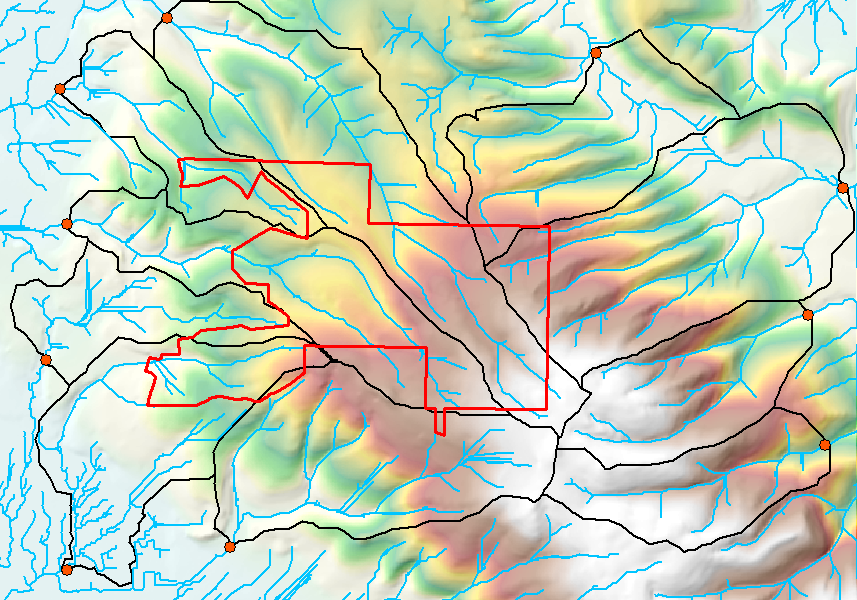
For your report, include a map of the watersheds, pour points, and streams. Use a nice hillshade but make sure to make the contract low or make it relatively transparent so it does not interfere with your key message. The one below is just to give an idea of the final map. Yours should include the required elements, labels, and look nicer!

 

Computing geometries

For our report, we need to include the number of streams, their length, and the number of watersheds, and their area. For the report, we'll be using the streams that drain at least 100 pixels (include the area of these headwaters in your report).

1. Open the attribute table (right click on the layer and select "Open Attribute Table".
2. Click on the little arrow in the upper left of the attribute table and select "Add Field".
3. 
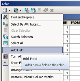
4. Name the field "Length". Note that the names of fields in ArcGIS are only allowed to be 10 characters long.
5. Set the "Type" to "Double".
6. Don't worry about the "Field Properties" now or even in the future. I never change these.
7. When you click "OK" the new field should appear.
8. Right click on the field heading and select "Calculate Geometry...". This will open a tool you can use to compute the length of polylines, the area of polygons, and to get the coordinate values for points.
9. 
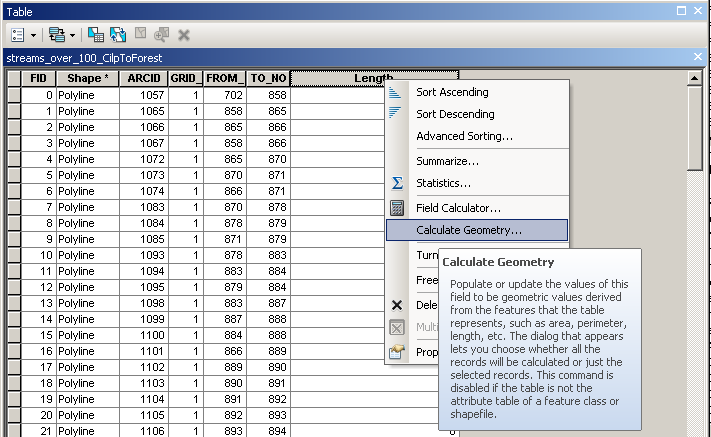
10. You may get an error at this point that you are outside an editing session. That is OK and just keep going.
11. Compute the "Length" of the streams

Other Resources

Esri Help