Music Festival, Part 2 - Musical Destination
Introduction
In the previous lab, we learned where to acquire data and how to perform a standardized quality assurance and quality control procedure. Now that we have the data, we will prepare it for analysis by projecting the data into the same projection and coordinate system. Once this is done, we will narrow down our choice of music festival locations using attribute selection methods and overlay operations. Our goal is to identify a festival site that is categorized as "Rural Residential", zoned as "U" or "unclassified", has a good access to roads and cell signal, but not encroaching on rivers or wetlands, and large enough for a good-sized crowd.
Learning Outcomes
- Use the " Project " tool to project data into the same spatial reference
- Add tabular x y data and convert to a shapefile
- Use basic vector analysis tools (Intersect, Buffer, Clip, Dissolve, Erase, Add Field, Field Properties, Select by Attribute, Boolean Operators, Select by Location (Spatial Selection), Field Calculator)
- Perform basic overlay operations: Intersect, Buffer, Clip, Dissolve, Erase
- Use Boolean operators to select features, create a new layer from selected features, and export selected features to a new shapefile
- Create maps that convey results of spatial analysis
Project Flowchart
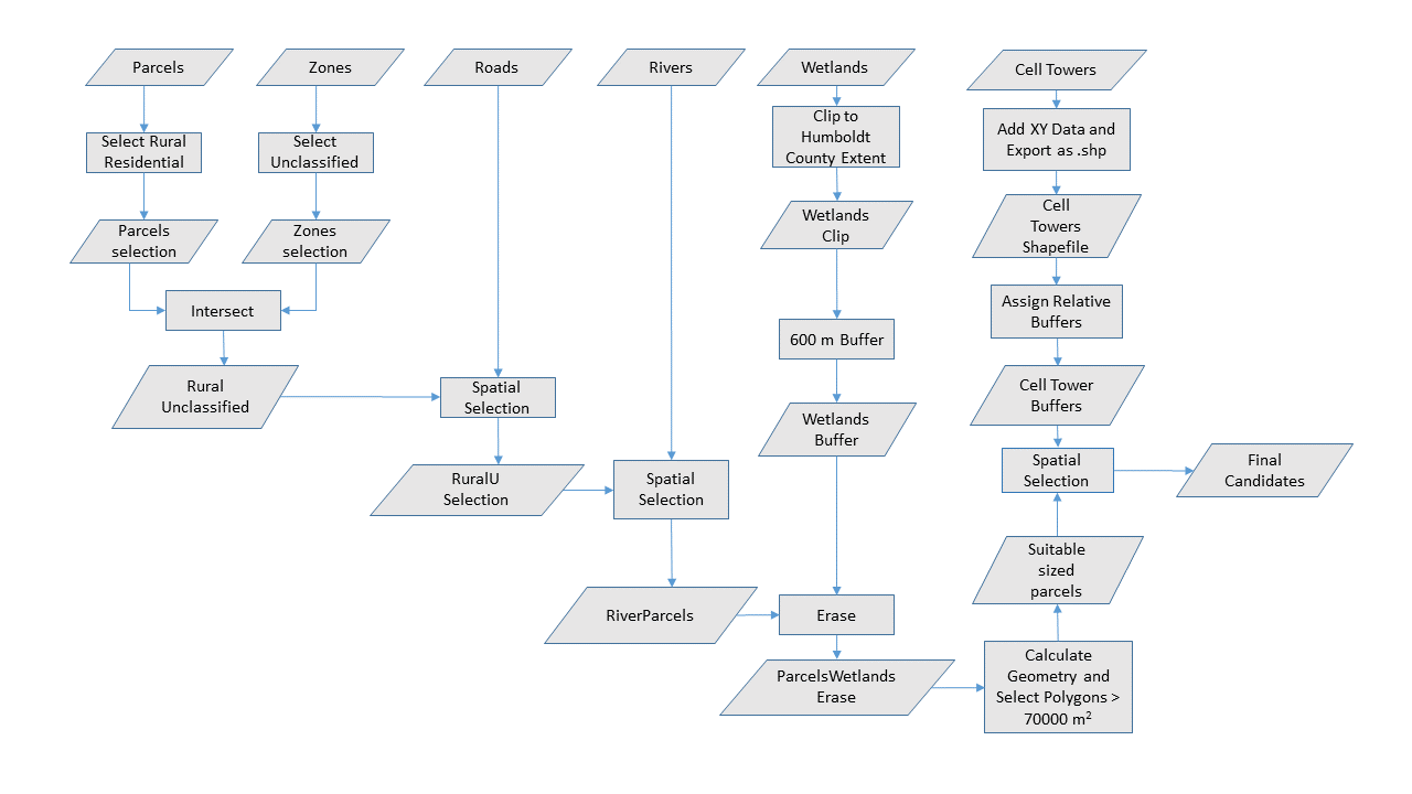
A flowchart is an easy-to-understand diagram that gives you the gist of the project in a single glance. This is a very good way of communicating and documenting your project quick and clear, so that the analysis will more likely be understood and applied correctly and consistently. By focusing on the detail of an individual step, identifying the input(s), analysis tool(s), and output(s) and how the elements are linked to one another, you also benefit from the process of creating a flow chart itself. Below is a flowchart summarizing our project to achieve the goal mentioned above.
Walk Through: Projecting Vector Data
It is important that each layer in any analysis you perform have the same spatial reference system. This will minimize uncertainty and error. Any error related to map projections will at least be uniform throughout the analysis if they all share the same spatial reference system.
In this step we will project each of our data sets into NAD83 UTM Zone 10 North. If you will recall from GSP 101, this is an international coordinate system based on the Transverse Mercator projection. It is particularly accurate for regions with a North/South orientation, such as Humboldt County. UTM always uses meters as the linear unit.
- Let’s begin by creating our standard workspace with the folders "Originals", "Working", and "Final".
- If you haven't already, download a copy of all the data sets for this lab to your orignals folder using these links: Music Festival II Data - No Wetlands and Music Festival II Wetlands Data. These are all the data sets downloaded in the previous lab, plus one additional dataset containing information on the cell towers. The data from the web sites you downloaded in the previous lab may have changed and we want to make sure you are successful in this lab so we've provided a set we know will work.
- Use the 7-Zip software to extract the zipped files.
- Launch ArcMap and open a blank map document (.mxd).
- Open the Catalog Tree and navigate to your originals folder.
- Drag and drop the file containing the rivers and streams onto your map. It may be called "nhd24kst_I_ca023.shp".
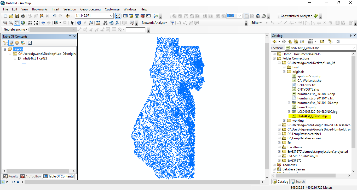
This first layer is already in the spatial reference system we want to use, NAD83 UTM Zone10N. However, we should check to be sure.
- Open the layer properties for "nhd24kst_I_ca023.shp" and check the spatial reference system.
- If the spatial reference system is correct, give the shapefile a more meaningful name. Right click on the shapefile "nhd24kst_I_ca023.shp"in the Catalog tree and select "Rename". Change the name to "rivers.shp".
Next, we will add the remaining shapefiles one at a time. You may ignore any "Geographic Coordinate Systems Warning" that may pop-up.
- Rename the shapefile "apnhum50sp.shp" to "parcels.shp" and add it to the map by dragging and dropping it from the Catalog tree.
- Rename the shapefile "CA_Wetlands.shp" to "wetlands.shp" and add it to the map.
- Rename the shapefile "CNTYOUTL.shp" to "county.shp" and add it to the map.
- Rename the shapefile "humtrans3sp_2013130417.shp" to "roads.shp" and add it to the map.
- Rename the shapefile "humz33sp.shp" to "zones.shp" and add it to the map.
- Leave the raster image of Humboldt County ("LC80460322015046LGN00") alone for now. We will get to that later.
We have now loaded each one of the six shapefiles. It is now time to use the "Project" tool to create copies of these files in the spatial reference system that we want, NAD83 UTM Zone 10 North. We could use the "Project" tool to create a copy of the shapefiles in the new spatial reference system one at a time. However, there is a script tool called "Batch Project" which allows us to load multiple files and project them all at once. It iterates though the list of loaded files and runs the "Project" tool for each one. To save time, we will use "Batch Project".
- Open the ArcToolbox by clicking on the red toolbox icon.

- Navigate to "Data Management Tools", "Projections and Transformations", and Double Click on the "Batch Project" tool to open it.
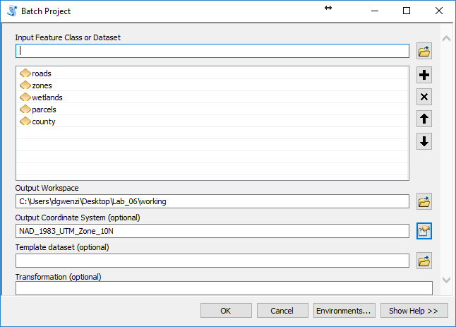
- Drag and Drop roads, zones, wetlands, parcels, and county into the lined window of the "Batch Project" tool as shown below.
Remember, the rivers layer is already in the projection we want. We don't need to project this shapefile.
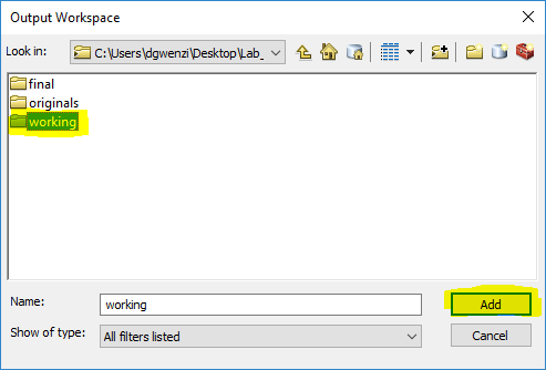
- The "Output Workspace" wants a folder, NOT a file. Use the yellow browse button on the right to navigate to your "working" folder. Select the working folder and click Add. See the image below.
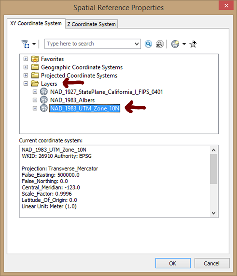
- Next to "Output Coordinate System" click on the icon to the right to choose the spatial reference system we want to use.
- Expand the "Layers Folder". This folder contains a list of all of the spatial reference systems currently in use by ArcMap. Since our "Rivers" shapefile has the spatial reference system we want and it is currently loaded on the map, "NAD 1983 UTM Zone 10N" will appear on the list. Select "NAD_1983_UTM_Zone_10N" and click OK. See the image below.
- Your "Batch Project" window should now look like the one below.
- Keep the remaining default settings and click OK.
Some of the files are rather large. It may take a few minutes to project them all. Please be patient.
Once the batch project tool is complete, you should see a copy of each of these layers in your "Working" folder.
Walk Through: Projecting Raster Data
Now that we have our shapefiles in the correct projection, we will do the same for our raster data. You will find that most tools require a separate set for raster and vector data. In this case we will use the "Project Raster" tool.
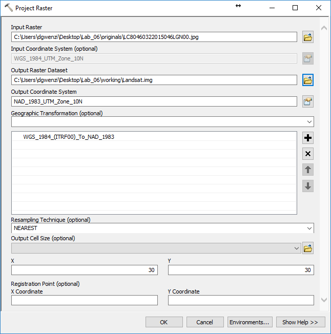
- Navigate to "Data Management Tools", "Projections and Transformations","Raster", and select the "Project Raster" tool.
- Drag and drop the LandSat image into the "Input Raster" field.
- For the "Output Raster Dataset" be sure to save to your working folder. Call the output "Landsat.img". The "img" or "Imagine" file format is the best file format for rasters when working with ArcGIS.
- For the "Output Coordinate System", open the Spatial Reference Properties window by clicking the icon on the right. Just as before, we will use the "Layers" folder to select "NAD_1983_UTM_Zone_10N".
- Leave the remaining default settings as they are and click OK. See the image below for clarification.
Walk Through: Adding XY Data
Before we start, lets be sure that our map data frame, labeled "Layers" in the Table of Contents is in the correct spatial reference system.
- Right click on the word "Layers" in the Table of Contents and select "Properties".
- Click on the "Coordinate System" tab.
- Make sure the Current Coordinate System is set to "NAD_1983_UTM_Zone_10N". If not, make the change yourself.
In this next step we will add the cell tower data, which is in the form of a tab delimited text file. We will add this file as "X Y data" and Define the projection as we add it it. The result will be a temporary "events" layer that we will have to export as a shapefile.
- First lets take a quick look at the data. In the Catalog Window, in your originals folder double click "CellTower.txt". This should open the file in a simple text editor as shown below.
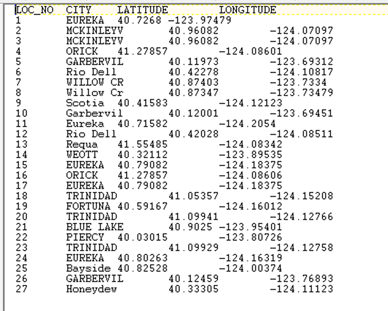
As you can see, the data is quite simple. It is in a "tab delimited format", which means that it is in a table where each column is separated by a tab. The column headers are "Loc_No", "City", "Latitude", and "Longitude". It is the last two columns, Latitude and Longitude, that are necessary to place this information on a map. This is the "X Y" component of the data.
- From the Catalog Window, drag and drop the "CellTower.txt" file from the "Originals" folder, onto the map.
When the file is added, the Table of Contents changes. Instead of being in the "List by Drawing Order" mode, it changes to the "List by Source" mode. It is easy to miss if you are not watching carefully. It does this because tabular data is not "drawn" on the map. This file will not show up in the Table of Contents when in "List by Drawing Order" mode. For now, we need to keep it in "List by Source".
Note: You must change it back to "List by Drawing Order" if you want to be able to change layer visibility by dragging the layers up and down in the Table of Contents. For now, leave it as it is.
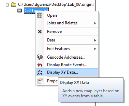
- Right Click on "CellTower.txt" in the Table of Contents and select "Display XY Data" as shown below.
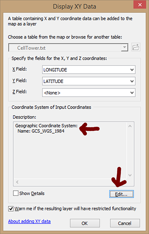
The display XY Data window is now open. The X field and the Y field are detected automatically. This is Longitude and Latitude respectively. However, ArcMap will try to define the projection using the same spatial reference system as the map data frame. This is most often the incorrect definition. The correct way to define the projection is to use the same spatial reference system that the data is currently in.
In this case, the Cell Towers were created using a Geographic Coordinate System, not a Projected Coordinate System. We must define it as "GCS_WGS_1984". See the image below for clarification.
- Click on the "Edit" button near the bottom right of the window. This will open the "Spatial Reference Properties" window, which by now should be familiar to you.
- Navigate to the "Geographic Coordinate Systems"by scrolling up to the top. Then locate the "World" folder" and select "WGS 1984". Click OK.
- If your settings look like the image below, click OK.
A warning appears "Table does not have object-ID field". This is warning you that though the layer may appear to be a valid vector file in the Table of Contents, it is not a shapefile. It will load as a temporary "events" layer. The ID field is a default numeric index that forces each row in the database to have a unique ID. This makes it possible perform queries and selections.
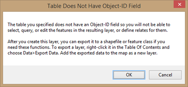
- Click OK to close the warning.
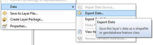
- Switch the "Table of Contents" to "List by Drawing Order" and Right click on the "CellTower.txt Events" layer and select "Data" then "Export Data".
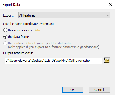
- Click on the radio button next to "the data frame" as shown below. This will project the data into NAD 83 UTM Zone 10 North at the same time it exports as a shapefile.
- Click on the yellow browse button to save the shapefile to your "Working" folder and name it "CellTowers.shp"..
- Click OK. See the image below for clarification.
- Click "Yes" to add to the map.
We now should have all of our layers ready and in the same coordinate system. We will start with a new blank map document (.mxd) and load only the necessary layers we are going to use in order to avoid confusion.
- From the "File" menu near the upper left corner of ArcMap, Select "New".
- Choose "Blank Map" if prompted and click OK.
- Click "No" when it asks to save the previous mxd.
Walk Through: Attribute Query
Within the "Parcels" shapefile, there are polygons that have been categorized as Rural Residential. These categorizes are stored in the attribute "EXLU4" in the attribute table. To only select these polygons, we must use the "Select by Attributes" tool within ArcMap. In this section, we'll show you how to use the tool and then you'll use it on your own in the next section.
- From the Catalog window, navigate to your "Working" folder and drag and drop the "parcels.shp" onto the map.
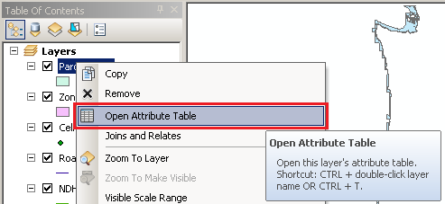
- From the Table of Contents, right-click on "Parcels" and click on "Open Attribute Table:"
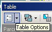
- Within the Attribute Table, select the small arrow in the upper left that contains, "Table Options":
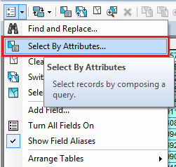
- From the drop-down menu, click on "Select by Attributes":
- This next step will bring up a "Select by Attributes" window.
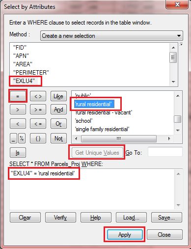
- Double-click on "EXLU4" within the box under Method (notice that "EXLU4" appears in the box at the bottom),
- Click on "Get Unique Values".
- "Get Unique Values" will populate all unique values in the attribute column "EXLU4" within the middle box.
- Click on the equals sign ("=").
- Double-click on 'rural residential' (notice that this text will appear in the box at the bottom). Your window should look like the one depicted below (without the red boxes).
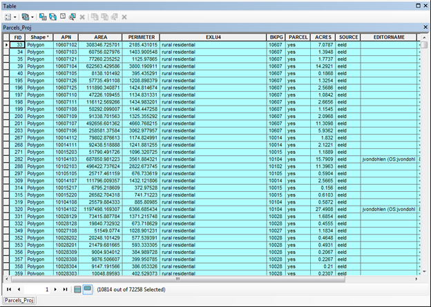
- Click on "Apply" and all fields that match this description should highlight within the Attribute Table:
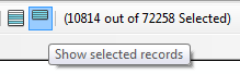
- Click on "Show selected records" at the bottom of the attribute table window to only view selected records within the Attribute Table:
We can now export the current selection as a new dataset. In other words, we will subset the data to create a layer with only those records that we are interested in.
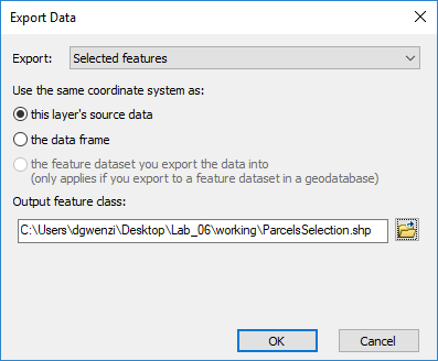
- With the current selection, in the Table of Contents, right-click on "Parcels" and select "Data" then "Export Data". For "Export:" choose "Selected features" and for "Use the same coordinate system as:", select "this layer's source data". Click the folder icon under "Output feature class:" then save the shapefile to your working folder and name it "ParcelsSelection.shp". See the image below for clarification.
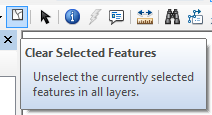
- Click "OK" and when prompted, click "Yes" to add the exported data to the map as a layer. Within the Tools Toolbar above the Table of Contents, click on "Clear Selected Features" on the toolbar.
Skill Drill 1: Attributes Query
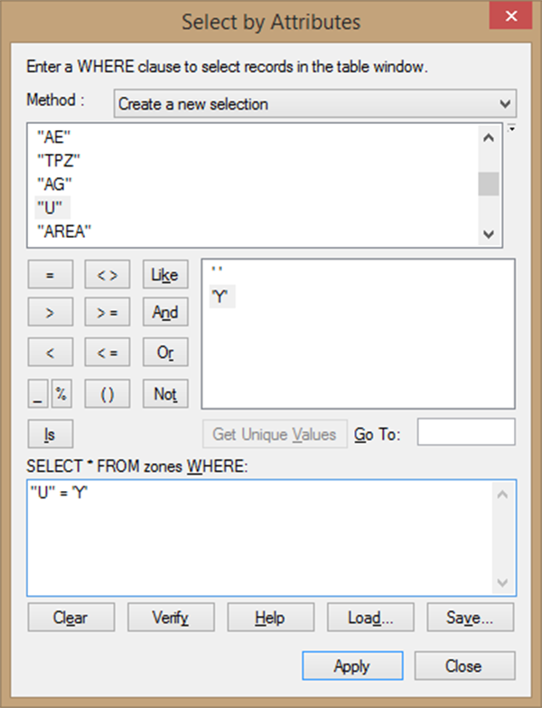
Select Areas that are Zoned as "U"
The next section will have you select the areas of Humboldt County that are zoned as "U" or "unclassified".
- Drag and drop the "zones" shapefile from the working folder onto the map.
- Open the attribute table for the "zones" layer.
- Select by Attributes for all features with a 'Y' (Yes) in the "U" attribute.
- In the Table of Contents, right click on "Zones" and export the selected records like you did for parcels. Save the shapefile to your working folder and name it "ZonesSeletion.shp". Click "Yes" to add the exported data to the map as a layer.
- Clear your selection as before
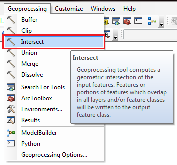
Walk Through: Performing an Intersect Overlay Operation.
- From the menu near the top of ArcMap select "Geoprocessing", then "Intersect".
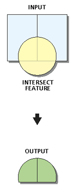
By using the Intersect tool on the Zoning and Parcels selection layers, you are producing a shapefile that contains an Attribute Table that has all instances where a polygon is both 'U' and 'Rural Residential.'
An Intersect generates a shapefile with a "geometric intersection" of the input features. All overlapping features are combined, while non-overalapping features are eliminated. See the graphic below.
- Drag and Drop the "ZonesSelection" and "ParcelsSelection" layers to the lined window on the Intersect tool.
- For "Output Feature Class," navigate to your working folder by clicking on the folder icon and saving your output shapefile as "RuralU.shp:"
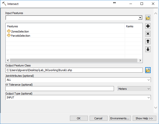
This will create a new layer, "RuralU" that contains only features that are rural residential and zoned as "U".
We no longer need our selection layers, the parcel layer, or the zone layer. All we need is our new "RuralU" layer. To keep things organized, remove them from the Table of Contents.
- Right click on all of the layers except "RuralU" and select "Remove". Only "RuralU" should be loaded onto the map.
Walk Through: Spatial Query
Next, we want to select all the areas that overlap with a road.
- From the Catalog Window, drag and drop "roads.shp" from your working folder, onto the map.
- To select all features within "RuralU" that overlap with the roads shapefile, you can use "Select by Location"
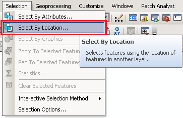
- Click on the "Selection" tab and click on "Select By Location" from the drop-down menu:
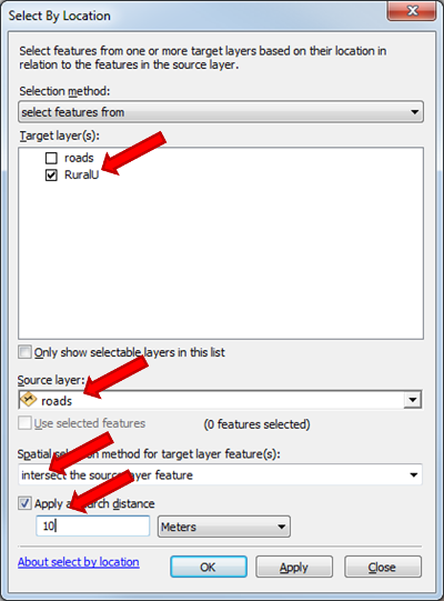
- Check the RuralU box within the "Target Layer(s)".
- Click on roads within the "Source Layer" drop-down menu.
- Make sure "intersect the source layer feature" is the chosen "Spatial selection method for target layer feature(s):". See the image below for clarification.
- You'll also need to check "Apply a search distance" and enter 10 meters for the distance.
- Leave all other options as default and click "OK".
- In the Table of Contents, right click on "RuralU" and export the selected records like you did with the earlier data sets. Save the shapefile to your working folder and name it "RuralUselection.shp". Click "Yes" to add the exported data to the map as a layer..
- Clear the selected features
- We no longer need the "roads" and "RuralU" layers. In the "Table of Contents", right click and remove them.
Skill Drill 2: Spatial Query
Our Final Parcel cannot intersect with any rivers or water bodies, so the following steps will produce a selection of all areas in our "ruralU selection" layer that do not overlap with the National Hydrology Database (NHD) and the Wetlands data.
If you will recall, the rivers shapefile was already in the spatial reference system NAD 83 UTM Zone 10 North, so it is still located in our originals folder.
- From the Catalog Window, drag and drop "rivers" from the originals folder onto the map.
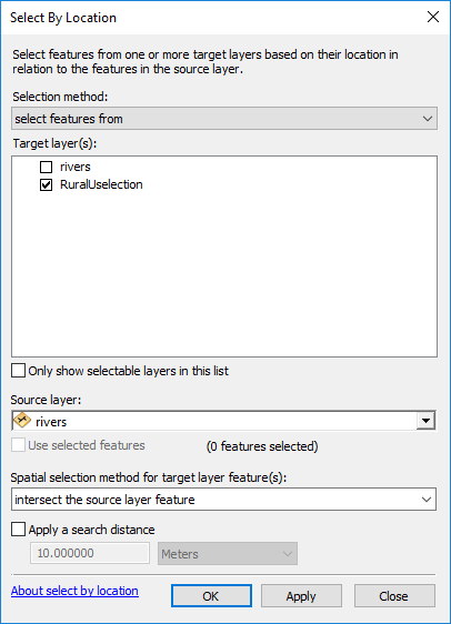
- Use what you learned in the previous walk though about spatial selections to select all features from our "RuralUselection" layer that intersect with the rivers layer. See the image below for clarification and remember to remove the "Apply a search distance" option.
- Once the layers are selected, open the attribute table for the "RuralU selection" layer.
- Click on the "Switch Selection" button to reverse the selected features.
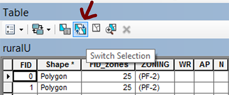
Switch Selection deselects all attributes currently selected and selects the remaining attributes that were not selected from the original query.
- Export the selected records to your working folder and save the file as "RiverParcels.shp".
- Clear selected features.
- Remove the "rivers" and "RuralUselection" layer from the Table of Contents, keeping only "RiverParcels".
Walk Through: Clip
To work with the wetland data, we'll need to clip the wetlands just to Humboldt County, then buffer the area around the wetlands, and then erase the remaining area from our current layer.
- From the Catalog Window, drag and drop the "wetlands.shp" and "county.shp" files from the working folder.
- From the Catalog Window, drag and drop the "county.shp" from the working folder.
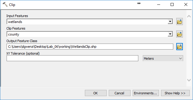
- From the Geoprocessing menu, select Clip.
- We want to "clip" to wetlands file so drag and drop it into the "Input Features".
- We want to use the Humboldt County layer to clip the wetlands so drag the county outline to the "Clip Features" box.
- For the "Output Feature Class", navigate to your working folder and name the file "WetlandsClip.shp".
- Leave all the remaining default settings as they are and click "OK". See the image below for clarification.
- Once the clip operation is complete, you may remove the wetlands and county layers from the Table of Contents.
The wetlands shapefile is large so this operation may take a while. Please be patient.
Walk Through: Buffer
We will utilize the Buffer tool to place our Music Festival 600 meters from any wetlands within Humboldt County.
- Select "Buffer" from the "Geoprocessing" menu.
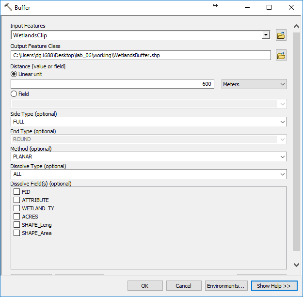
- Drag and drop the "wetlandsClip" to the "Input Features".
- For the "Output Feature Class" navigate to your working folder and name the file "WetlandsBuffer".
- Next to "Distance [value or field], you have two choices. You can set the buffer to a fixed distance or use an attribute field to define the buffer distance. In this step will will use a "Linear unit" and enter "600" for 600 meters.
- Next to "Dissolve Type" use the drop down menu and select "ALL".
- Leave all remaining settings at default. See the image below for clarification.
- Click "OK" and when this is done you may remove wetlands_clip from the Table of Contents.
This operation may also take a while, possibly 5 to 10 minutes. Please be patient. You may want to take this time to get up and stretch, get a drink of water, or walk around for a bit.
Walk Through: Erase
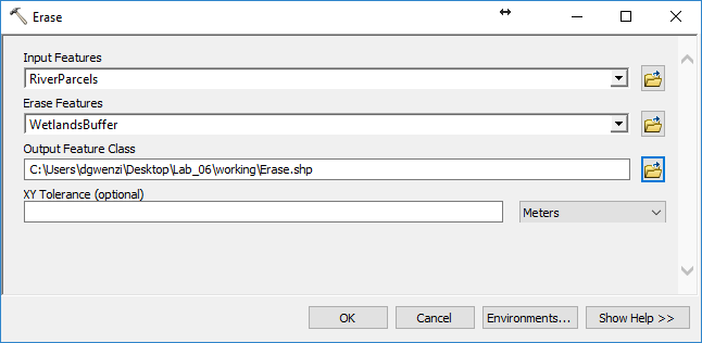
In this next step we will use our "WetlandsBuffer" to erase. This tool is fairly straight forward, in that it will erase all of the area covered by the wetlandBuffer from RiverParcels.
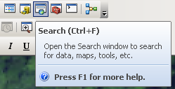
The Erase tool is not located in the Geoprocessing menu. We will have to search for it.
- Click on the Search button to open a search window:
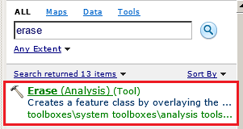
- Type in "erase" and hit [Enter], then click on the first option Erase (Analysis):
- Input "RiverParcels" as the Input Features, and "WetlandsBuffer" as the erase features and save your output shapefile as "Erase.shp."
- Click "OK" to execute the "Erase" tool. Once the process is done, you may now remove both the "RiverParcels" and "wetlandsBuffer" from your Table of Contents.
Skill Drill: Calculate Geometry and Attribute Selection
We have met most of our criteria so far, however we want to weed out very small parcels and sliver polygons left over from our erase operation.
However, whenever you perform an overlay operation like "clip", "intersect", or "erase", the area values recorded in the attribute table are not automatically updated. They still have the original values, which are now incorrect. In order to determine which areas to keep, we will need to update the "Area" field by using Calculating Geometry.
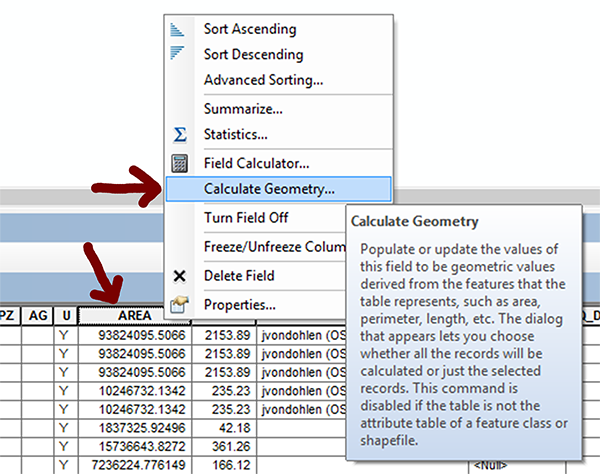
- Open the attribute table for the "Erase" layer.
- Find the "Area" field and right-click on the word "Area".
- Select, "Calculate Geometry".
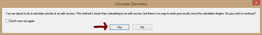
- You will see a warning. This message means that you are about to edit the shapefile outside of an "edit" session. Any change you make is a permanent change to the shapefile that cannot be undone. This is fine, so go ahead and click "yes".
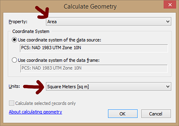
- The Calculate Geometry window opens up and it is here that you can determine the property and units. In this case we want our "Property" to be set to "Area" and our "Units" to be set to "Square Meters". See image below for clarification.
- After you click OK, ArcMap feels the need to warn you a second time. Click Yes.
Now that we know the square meters in the Area field are updated, we want to select parcels with an area greater than seventy thousand (70000) square meters.
- Use "Select by Attributes" to select the records with an area that is greater than seventy thousand square meters. "Select by Attributes" is like a calculator but it does not understand commas in numbers so you can just use:
"Area" > 70000
- All the selected records should be greater than 70000 square meters. Export these records as a shapefile into your working folder and name it "EraseSelection". Once this is done, you may now remove the Erase layer from the Table of Contents
Walk through: Using the Field Calculator to Populate Values within a Field.
Our music festival will require a stable signal from a cell tower. In this scenario we have been given data on the range of certain cell towers. For the next series of steps, we will be creating buffers based on these different ranges. We will need to create a field within the attribute table of our cell towers to hold these buffer distance values. We will do this by selecting the appropriate cell tower locations and using the Field Calculator to assign values to selected records.
- From the Catalog Window, drag and drop the "celltower.shp" from the working folder.
- Open the attribute table for the "celltowers" layer.
- From the Table Options drop-down menu (upper left on the attribute table), click on Add Field:
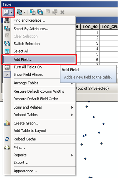
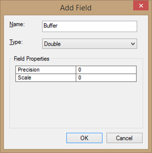
- Fill in the Name as "Buffer".
- Select "Double" from the drop-down menu next to "Type"
- Leave the remaining settings as default and click OK.
The table below shows the buffer values that need to be assigned to each cell tower. These buffers represent the stable signal range of those towers.
| Towers ("LOC_NO") |
Buffer |
| 7-8,21,25 |
400 |
| 5-6,9-12,14,18,22,26-27 |
1000 |
| 1-3,15,17,19-20,23 |
5500 |
| 4,13,16,24 |
8000 |
In the next series of steps we will use Select by Attributes to select a range of cell towers. Once the cell towers are selected, we will run the Field Calculator. This tool will only update the records (rows) that are selected (highlighted) by our Select by Attributes.
Lets start with the first row. We will select cell towers with a location number of 7,8,21, and 25.
- Open the "Select by Attribute" window and enter the following expression:
("LOC_NO" >= 7 AND "LOC_NO" <= 8) OR ("LOC_NO" = 21) OR ("LOC_NO" = 25)
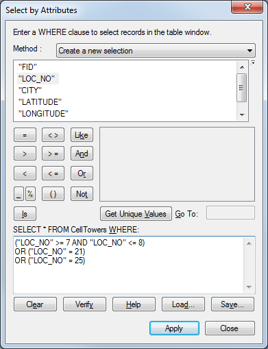
Take a look at the line of text above our expression that reads "SELECT * FROM celltowers WHERE:". This is part of a Structured Query Language or "SQL" statement. Our expression completes this statement. SQL is the standard language for relational databases and is also used within ArcGIS.
Take a moment and work through the logic of the SQL query. It will select records where the value in the location number field meets the conditions of being both less than or equal to seven AND ALSO less than or equal to eight. Both conditions must be true when using the AND operator. The numbers 7 and 8 meet both these conditions, so both records will be selected.
Now an OR is added afterwards. This means that if it does not meet the first condition, it may also be selected if the location number equals 21 or if the location number equals 25. Either condition can be true with an OR operator.
Note that after each Boolean Operator (AND, OR) a complete SQL statement is required. This means it must include the field name ("LOC_NO"), a comparison operator (<,>,=, <=, >=), followed by a value. If you try to take a short cut with SQL syntax and leave something out, it will not work!
Click "Apply". Now that the cell towers with a range of 400 meters are selected we can use the field calculator to enter the number 400 in each of these selected records.
- In the attribute table, right-click on the name "Buffer" and select "Field Calculator".
- Click "Yes" when the warning appears.
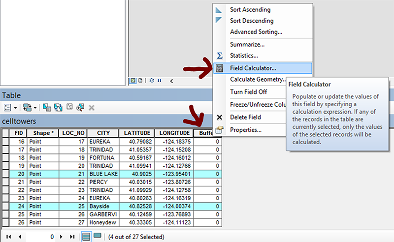
- Under "Buffer = ", enter 400 and click on "OK"
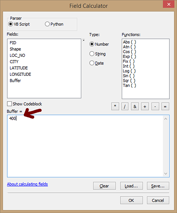
Field Calculator does not use SQL. It can use VB Script or Python. Note that the code begins just above the number 400 in the image above with the words "Buffer =". The complete statement reads "Buffer = 400".
The results of the field calculator on the selected records is shown below.
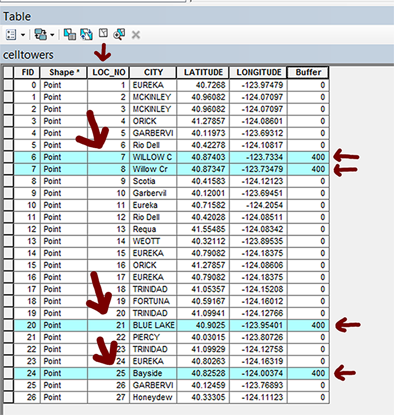
As you can see the field calculator only works on selected records.
Skill Drill: Attribute Selection Followed by Field Calculator.
Now you can repeat the steps above until the buffer values from the table have all been applied to the celltower Attribute Table.
| Towers ("LOC_NO") |
Buffer |
| 7-8,21,25 |
400 |
| 5-6,9-12,14,18,22,26-27 |
1000 |
| 1-3,15,17,19-20,23 |
5500 |
| 4,13,16,24 |
8000 |
Hint: When writing your SQL statements for the Select By Attributes window, think of the dashes on the table as "AND"s and the commas on the table as "OR"s.
- Repeat the steps above until the buffer values from the table above have all been applied to the celltower Attribute Table.
Skill Drill: Create a Buffer based on a Field
In this step you will create a buffer. Instead of using a linear unit as before, we will chose to use the Buffer field in the celltower attribute table.
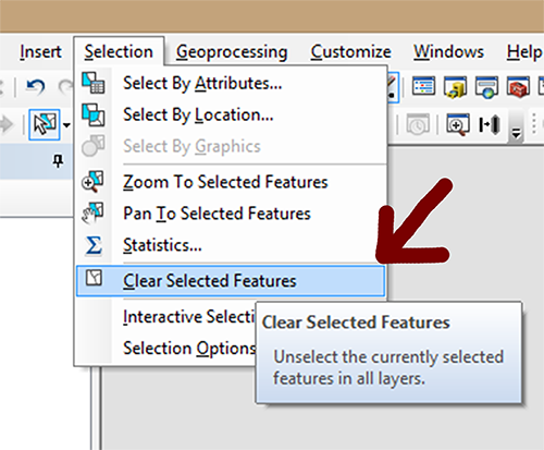
Before you run the buffer too you MUST clear select features. If you don't, the buffer will only work on the cell towers currently selected.
- From the top menu click "Selection" then "Clear Selected Features".
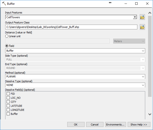
- From the Geoprocessing drop-down menu, click on Buffer.
- Drag and drop the "celltowers" layer into the Input Features
- Navigate to your working Folder to save your shapefile as "CellTower_Buff".
- Click on the "Field" radio button.
- From the drop-down menu within "Field", select "Buffer".
- Leave all other options at default and click on OK. See the image below for clarification.
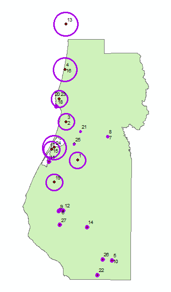
You result should be a layer composed of variable distance buffers, similar to the image below.
Skill Drill: Spatial Selection to Determine Potential Sites
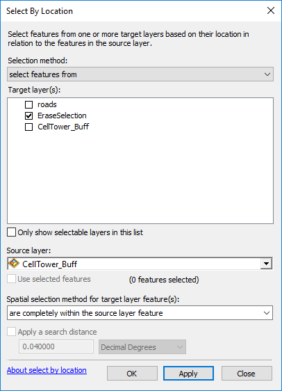
For the final step we will narrow down our list of potential sites by determining which parcels fall within the range of the cell towers. To do this we must perform a spatial selection to identify the parcels in the "EraseSelection" layer that are completely within a cell tower range.
- From the ArcMap main menu, click on Selection, then Select By Location and specify the Target layer, Source layer and Spatial selection method as shown below.
- Exported the selected features and save the output as "FinalCandidates.shp"
- You may now remove all other layers from the Table of Contents and leave only the FinalCandidates layer
- Now is a good time to save your .mxd!
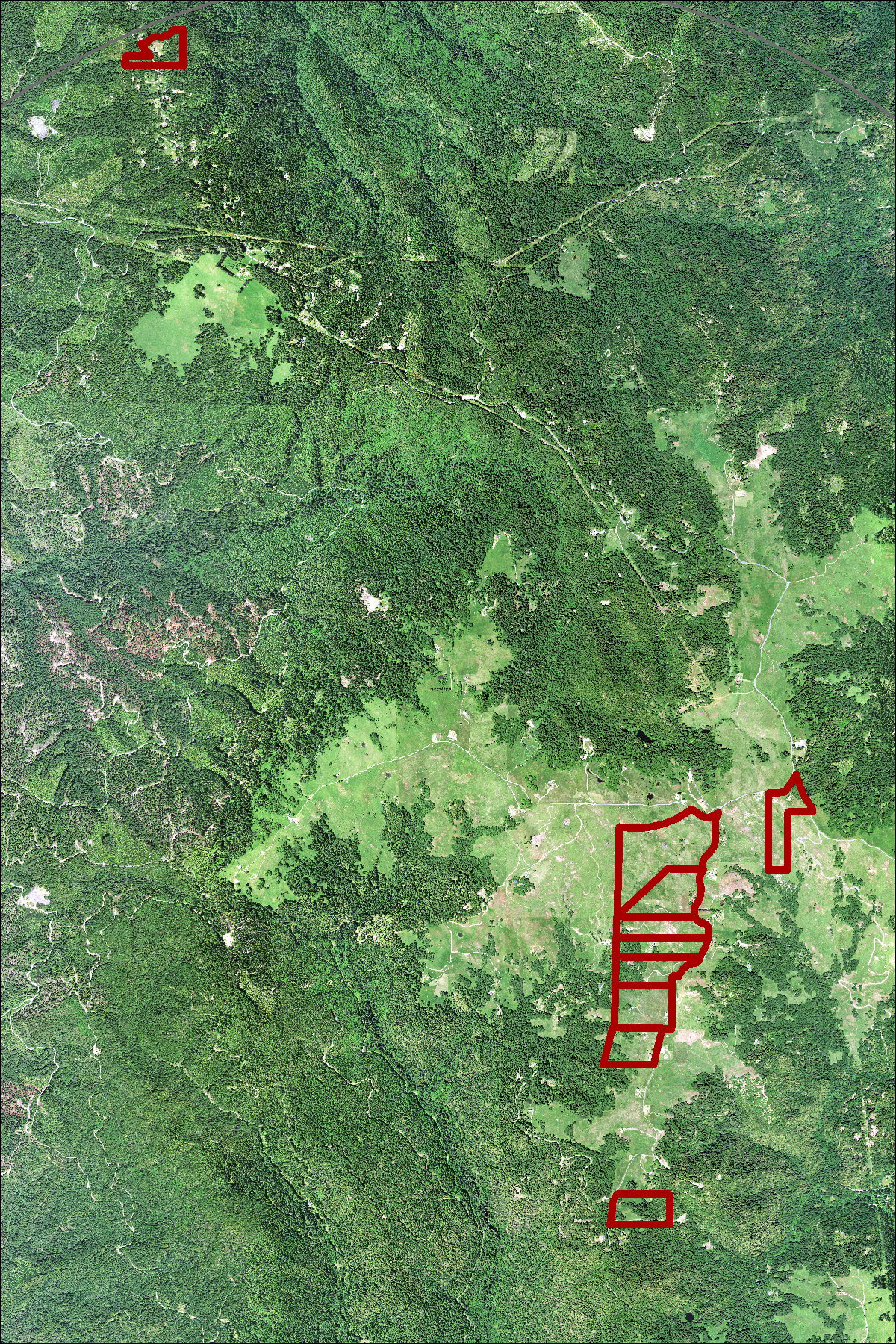
The final result should be a small group of parcels that will be our potential Music Festival sites. If you had a background, it should appear as shown in the image below.
Remember to back up your data. When using the Google Drive, click the link below for a video that will show you how to make sure your data is completely backed up before you log out.
Using Google File Stream