Categorical and Regression Trees

Under Construction

Loading the Libraries

Tree models are the most natural method to model response variables that are categorical (i.e. soil type, land cover type, etc.). However, they can also be used to model continuous responses but be careful of over fitting.

CART results additional libraries to be loaded into R as shown below. You only need to execute this code once in R-Studio.

install.packages("tree")
install.packages("rpart")

You will need to add the library's "tree" and "rpart" to your script:

library(tree)
library(rpart)

The MSU Lab

There is an excellent treatment of CART with a tiny data set at: http://ecology.msu.montana.edu/labdsv/R/labs/lab6/lab6.html

Doug-Fir Examples

The following examples were created using the Doug-Fir data we extracted from the FIA database.

TheData <- read.csv("C:/ProjectsModeling/Cali_5Minute/DougFir_CA_Predict 4.csv")

# Remove any NA (null) values, the data should already be loaded
TheData=na.omit(TheData)

Trees for Presence/Absence Data

Note: The material below is for the "tree()" function. This is no longer used as often as rpart() but it is easier to intepret the results.

There are two methods for creating tree models with presence/absence data, one will return a probability of presence and the other will return TRUE for presence and FALSE for absence. We'll look at TRUE/FALSE first but to achieve this, we need to add a "factor()" function and a Boolean equation so that the tree() function sees variables that are TRUE or FALSE. The code below will create the tree.

TheModel = tree(factor(TheData$Present>0)~TheData$AnnualPrecip+TheData$MinTemp)

To see a plot of the tree, we need to first draw the tree and then add text labels to the tree.

plot(TheModel) # Plot the tree
text(TheModel) # Add labels for the values at the branches

The tree shows us exactly how the tree will classify values. The length of the "branches" is an indication of the relative amount of "deviance" explained by each branch. We can see statistics for the model by using summary().

summary(TheModel)

The summary is a little different and is shown below.

Classification tree:  
tree(formula = factor(TheData$Present > 0) ~ TheData$AnnualPrecip + TheData$MinTemp)  
Number of terminal nodes: 6 Residual mean deviance: 0.358 = 2089 / 5834   
Misclassification error rate: 0.09658 = 564 / 5840

"Number of terminal nodes" is the number of "leaf" nodes in the tree and is a direct representation of the complexity of the tree as each time we add a branch, we add a "terminal node".
"Residual mean deviance" is the "Total residual deviance" divided by the "Number of observations" - "Number of Terminal Nodes".
- "Total residual deviance" is the sum of squares of the residuals
"Misclassification error rate" is simply the number of observations that were misclassified divided by the total number of observations.

Note: I recommend using the "Number of terminal nodes", the "Total residual deviance" to compare models, and the "Misclassification error rate" to evaluate models.

If you just enter the name of the model, you'll see the tree in text form.

node), split, n, deviance, yval, (yprob)
      * denotes terminal node

 1) root 5840 4902.00 FALSE ( 0.85171 0.14829 )  
   2) TheData$AnnualPrecip < 837 4524  859.80 FALSE ( 0.98077 0.01923 )  
     4) TheData$AnnualPrecip < 505.5 3322    0.00 FALSE ( 1.00000 0.00000 ) *
     5) TheData$AnnualPrecip > 505.5 1202  624.40 FALSE ( 0.92762 0.07238 )  
      10) TheData$MinTemp < -29.5 492  433.60 FALSE ( 0.83943 0.16057 ) *
      11) TheData$MinTemp > -29.5 710   87.68 FALSE ( 0.98873 0.01127 ) *
   3) TheData$AnnualPrecip > 837 1316 1780.00 TRUE ( 0.40805 0.59195 )  
     6) TheData$AnnualPrecip < 1302.5 924 1281.00 FALSE ( 0.50649 0.49351 )  
      12) TheData$MinTemp < -85 62   10.24 FALSE ( 0.98387 0.01613 ) *
      13) TheData$MinTemp > -85 862 1192.00 TRUE ( 0.47216 0.52784 ) *
     7) TheData$AnnualPrecip > 1302.5 392  364.80 TRUE ( 0.17602 0.82398 ) *

These values are:

node: a unique number for the node in the tree
split: the equation used to branch at the node
n: the number of observations following the left-side of the branch
deviance: the deviance associated with that branch
yval: predicted value at the node
(yprob): the proportion of values in that branch that are absent and present
*: an asterisk next to a node indicates it is terminal

The "root" node does not have any splits so it has the maximum deviance. Each node there after, reduces the deviance.

Trees for Continuous Data

We can also use trees for continuous response.

TheModel = tree(TheData$Height~TheData$AnnualPrecip+TheData$MinTemp)

The statistics for these models are the same as above except the "yprob" value is no longer available because we do not have probabilities for categories.

node), split, n, deviance, yval
      * denotes terminal node

 1) root 5840 16490000  21.010
   2) TheData$AnnualPrecip < 935.5 4745  2348000   3.744
     4) TheData$AnnualPrecip < 837 4524  1147000   2.105 *
     5) TheData$AnnualPrecip > 837 221   940400  37.300 *
   3) TheData$AnnualPrecip > 935.5 1095  6596000  95.820
	 6) TheData$AnnualPrecip < 1346 757  4503000  80.650
      12) TheData$MinTemp < -75.5 59   142600  20.320 *
      13) TheData$MinTemp > -75.5 698  4127000  85.750 *       
	 7) TheData$AnnualPrecip > 1346 338  1529000 129.800 *

Cross-Validation

The library we are using contains a function to perform a 10-fold cross-validation on tree models. This means it will use 90% of the data to create a model and 10% to test it. Then, it will run the model again with a different 10% and repeat this 10 times, until all the data has been used as training and test data.

TheCrossValidatedModel = cv.tree(TheModel) 

plot()

The resulting plot shows the change in deviance as different number of terminal nodes were used.

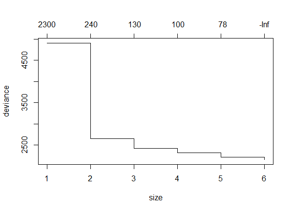
Note that the deviance goes down as the number of terminal nodes increases. This is not always the case.

Controlling the Number of Nodes

Typically, trees are over-fit to data. By default, the tree package will stop when each branch has less than 5 samples. With large datasets, this can make really large trees. You can control the number of nodes using the "prune" function. The "best" parameter requires only the best 4 nodes to be included.

PrunedModel <- prune.tree(TheModel,best=4)

Creating a Predicted Surface

We can create predictions for trees, either with existing or new data, using the "predict()" function. Note that to use new data with "predict()" we have to "attach()" the original data when creating the model, "detach()" the original data, then "attach()" the new data.

attach(OriginalData)
TheModel = tree(Height~AnnualPrecip+MinTemp)
detach("OriginalData")

attach(NewData)
ThePrediction=predict(TheModel,NewData)
detach("NewData")

Now you can add this prediction back into a data frame and save it to be loaded into a GIS application.

Additional Resources

R tree package

Tree Models in R

MSU Tree lab

R for Spatial Statistics