Generalized Additive Models (GAMs)

 

Creating a GAM Model

GAMs are an extremely powerful method for spatial modeling. GAMs add "smoothing" functions to the predictors to provide great flexibility in the nature of the response to the predictors.

Before starting below, you'll want to have a dataset that contains sampled values with associated predictor values. You'll also want to have a similar dataset setup with points covering the entire sample area and the predictor values in columns. Things will go easier if you have the names of the predictor values in both files matching exactly.

R makes creating GAMs extremely easy. The syntax is very similar to lm() with only a few additional parameters. To get started, you'll want to load the "mgcv" library and a data set into a data frame an use remove any null values.

require(mgcv) # load the GAMs library

# Read the data
TheData = read.csv("C:/ProjectsModeling/Cali_5Minute/DougFir_CA_Predict 4.csv")

# Remove any NA (null) values
TheData=na.omit(TheData)

To run a GAM, you provide a response variable and a series of predictor variables just as you did with a linear model. The difference is that you'll want to pass each predictor variable into an "s()" function for "spline". These functions will provide a smoothed spline curve. You'll also want to provide a distribution function for the response variable and a "link" function to link the response variable into the linear portion of the model. Typical functions are:

Type of data	Family of Distributions	Link Function
Continuous data	gaussian	identity
Binary data (true/false)	binomial	logit
0-based continuous	Gamma	inverse
Counts	poisson	log

 

The default family is "gaussian" and the format to specify the distribution is:

TheModel = gam(Height~s(AnnualPrecip),data=TheData,family=gaussian())
TheModel = gam(Height~s(AnnualPrecip),data=TheData,family=binomial()) 
TheModel = gam(Height~s(AnnualPrecip),data=TheData,family=Gamma()) 
TheModel = gam(Height~s(AnnualPrecip),data=TheData,family=poisson()) 

The last parameter that you will want to provide is a "gamma" parameter which specifies the amount of smoothing to apply to the spline curves. This can be interpreted as the number of "knots" used for the spline curves for each predictor variable. Below is an example.

To use the "predict.gam()" function to predict values from our model we will need to "attach()" the data set so the names of the columns can be matched between to the data set for the prediction.

Warning: after using a variable with "attach()" remember to detach it with "detach()". If you don't, the number of attached variables will continue to increase causing confusion and lots of warning messages. Also note that "detach()" requires that the variable name be in quotes. You can check the values that are attached with the function "search()".

# We have to use "attach()" because predicting values later on requires it
attach(TheData)

# the family is gaussian by default but the gamma should be changed from 1 to smooth
TheModel=gam(Height~s(AnnualPrecip),data=TheData,gamma=1.4) # Recommended smoothing factor

# remember to "detach()" the variable after using it
detach("TheData") # note the quotes

"summary()" provides similar values to a GLM except that we'll need to run the "AIC()" function to see the AIC value.

# The summary does not provide an AIC but "AIC()" does
summary(TheModel)
AIC(TheModel)

You can also get the likelihood for a GAM with:

logLik.gam(TheModel)

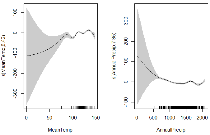
The plots are referred to as "partial dependence plots" because they only show the dependence between the predictor and response variables for one predictor. The standard "plot()" function will show the plots but you can also specify "pages=1" to have them all appear on one page.

# Plot the model, including confidence intervals
plot(TheModel)

# All the plots on one page
plot(TheModel, pages=1, scale=F, shade=T)

Below is an example output from a rather weak model (you can do better). The gray areas around the response curves are the confidence intervals. The "grass" at the bottom of the graphs shows the number of samples at each predictor values. The confidence intervals are very large on the left because the number of samples is also very low.

Creating a Predicted Spatial Surface

By default, the function "predict.gam()" will add predicted values to your existing dataset. You can also provide a different dataset with predictor values that include the entire sample area. If the headings for the files match the original file then the code below will produce new, predicted values.

# create a data set for the prediction (replace this with your predictor data set)
AnnualPrecip=as.vector(array(1:2000)) # create a vector with the full range of x values
NewData=data.frame(AnnualPrecip) # put this into a dataframe for prediction (names must match the model)

# create the prediction and plot it
Height=predict.gam(TheModel,NewData,type='response')
FinalData=data.frame(NewData,Height)
plot(NewData$AnnualPrecip,FinalData$Height)

# Save the prediction to a new file
write.csv(FinalData, "C:/ProjectsModeling/ModelOutput.csv") 

Now you can convert the prediction into a new layer in a GIS package. Remember to use the original extent and pixel size for the raster.

Vewing the GAMs with the correct Y-Axis

You've probably noticed that the Y-Axis with GAMs is not what you would expect. This is because the plots only show the contribution to the model for one predictor at a time. This does not include the Y-Intercept value. You can see this by fitting the original data to the model with the "fitted()" function.

plot(TheData$MaxTemp,fitted(TheModel))

Plotting GAMs in 3D

This was a bit of a challenge but the code below will create 3d graphs for a GAM with two covariates. It will also create GAM for each dimension to be compared with the overall GAM charts.

require(mgcv) 
require(rgl)

########################################################################################
# Function to create 3d polynomial-based data with noise injection
#
# Inputs:
# - NumEntries: the number of data values that will be produced
# - RandomStdDev: the standard deviation for noise injection (0=none)
# - X1B0: The y-intercept for 1st dimension
# - X1B1: Slope of the line for 1st dimension
# - X1B2: Second order coeficient for 1st dimension
# - X2B0: The y-intercept for 2nd dimension
# - X2B1: Slope of the line for 2nd dimension
# - X2B2: Second order coeficient for 2nd dimension
#
# Outputs a list containing:
# - [[1]]=The matrix with the z values. Size of the matrix is [NumEntries,NumEntries]
# - [[2]]=X1 indexes ranging from 1 to NumEntries for accessing the z values as a vector
# - [[3]]=X2 indexes rangnig from 1 to Numentries for accessing the z values as a vector
########################################################################################
Poly3DMatrix=function(NumEntries=100,RandomStdDev=0,X1B0=0,X1B1=0,X1B2=0,X2B0=0,X2B1=0,X2B2=0)
{
# for debugging:
# NumEntries=100
# RandomStdDev=0
# X1B0=0
# X1B1=0
# X1B2=0
# X2B0=0
# X2B1=0
# X2B2=0

# Create a 2d matrix for the z-values
Measures=matrix(nrow=NumEntries,ncol=NumEntries) 

# Compute the total size of the matrix
TotalEntries=NumEntries*NumEntries 

# Create the vectors to accompany the matrix
DataX1=as.vector(array(1:TotalEntries))
DataX2=as.vector(array(1:TotalEntries))

Index=1 # Overall index into vectors
X1=0 # Index in the x direction
while (X1<NumEntries) # Loop through the rows in the matrix
{
X2=0 # index in the y direction
while (X2<NumEntries) # loop through each cell in the current row
{
# add values to the vector
DataX1[Index]=X1+1
DataX2[Index]=X2+1
Index=Index+1

# Compute the z values
Measures[X1+1,X2+1]=X1B0+X1B1*X1+X1B2*(X1**2)+X2B0+X2B1*X2+X2B2*(X2**2)

X2=X2+1 # Move to the next cell in the row
}
X1=X1+1 # Move to the next row 
} 
# If desired, add some random noise to the matrix
if (RandomStdDev>0) # if a random value was provided
{
Measures=Measures+rnorm(TotalEntries, 0, sd = RandomStdDev)
}
Test=as.vector(Measures)

# return the data as a data frame
TheDataFrame = data.frame(DataX2, Test)
TheDataFrame$DataX1=DataX1

return(TheDataFrame)
} 
########################################################################################
# Code sample to create a matrix with two covariates based
# on a polynomial, fit a GAM, and plot it in 3D
# 
# Plotting code from: 
# https://www.rdocumentation.org/packages/rgl/versions/0.97.0/topics/surface3d
########################################################################################

# Setup the settings for the matrix
NumEntries=20 # The matrix will be NumEntries x NumEntries in size
RandomStdDev=20 # Amount of random noise to inject

# Create vectors to access the matrix in each dimension (x and y)
X1s=as.vector(array(1:NumEntries))
X2s=as.vector(array(1:NumEntries))

# Get the matrix of z values with x and y vectors that match the matrix as a vector
TheData=Poly3DMatrix(NumEntries,RandomStdDev,X1B0=10,X1B1=20,X1B2=0,X2B0=10,X2B1=-10,X2B2=3)
Measures=TheData$Test
DataX1=TheData$DataX1
DataX2=TheData$DataX2

# Plot the data in each dimension
par(mfrow=c(1,2))
plot(DataX1,Measures,main="Response for X1")
plot(DataX2,Measures,main="Response for X2")

# Create a 3D plot of the data
plot3d(DataX1,DataX2,Measures, col="red", size=10)

# Create a GAM for the data
TheModel=gam(Measures~s(DataX1)+s(DataX2),gamma=1.4) 
plot(TheModel)

# Create a gam for each direction independently
TheModelX1=gam(Measures~s(DataX1),data=TheData,gamma=1.4) 
plot(TheModelX1)

TheModelX2=gam(Measures~s(DataX2),data=TheData,gamma=1.4) 
plot(TheModelX2)

Predicted=predict.gam(TheModel,TheData,type='response')

# Create a Color-Look-up-Table (colorlut) for the predicted values

zlim <- range(Predicted)
zlen <- zlim[2] - zlim[1] + 1

colorlut <- terrain.colors(zlen) # height color lookup table

col <- colorlut[ Predicted - zlim[1] + 1 ] # assign colors to heights for each point

# plot our original data points
plot3d(DataX2,DataX1,Measures,col="red",size=10)

# plot our suface with the original data points
surface3d(X1s,X2s,Predicted, color = col, back = "lines")

Additional Resources

Original Paper on GAMs

R Package: Generalized Additive Models with Integrated Smoothness Estimation

Excellent Book on linear modeling: Generalized Additive Models: an introduction with R

Slide Presentation: Introduction to Generalized Linear Models

An introduction to mgcViz: visual tools for GAMs - examples of creating very nice graphics for GAMs.

GAM: The Predictive Modeling Silver Bullet - Details on how to fit maps