Lab 2- Part 2: Masking, Spectral Indices & Image Visualization

Introduction

In this lab we will cover techniques for masking and visualizing data in ENVI and ArcGIS Pro.

Learning Outcomes

• Download SRTM DEMs in ENVI
• Importing satellite imagery and data into ArcGIS Pro
• Evaluating Image Statistics and histograms
• Visualizing data in ArcGIS Pro
• Creating hillshades and other surface derived layer
• Creating maps from remotely sensed data

About the Data
The primary data for this lab is Landsat Collection 2 Level-1 and Level-1 data that has been calibrated and corrected to Surface Reflectance in the previous lab exercise. We will also use the Landsat Pixel QA bands that are supplied with the Level-1 and Level-2 data.

Opening Data and Accessing Tasks in ENVI

You will begin by copying over your Lab 2 Final data folder from the previous lab. ENVI Custom Tasks can be created using the ENVI Modeler. These tasks can be saved and added to the Toolbox in ENVI. When ENVI is launched it will automatically scan specific folders for custom tasks.

1. Begin by copying over your Lab 2 Final data folder (from the previous lab) to the desktop. You will need the two surface reflectance files (Level-1 and Level-2) and the Landsat QA bands (these are also available in the lab data folder on google Drive and Z: Drive separately).
2. Start ENVI and open both of your Surface Reflectance Landsat images. These files were generated in the previous lab exercise and represent the surface reflectance data.
3. Review the statistics for the Level-1 Surface Reflectance data (Surface_Reflectance.dat). Note that there are still values greater than 1 (100%) reflectance in this dataset. We need to "clip" the values outside the expected range using the High Clip task. In the last lab exercise we created a model to clip both the high and low values, but you can also call the ENVI task to run the tool.
4. Navigate to the Toolbox >Task Processing >Run Task. This will bring up the list of ENVI Tasks and Custom Tasks that can be run. Find the High Clip task and run it. Clip the values greater than 1 in all seven bands and save the file as Surface_ReflectanceL1.dat. Check the Quick Stats when you are done to confirm that there are no values outside the expected range.
5. Review the two final Surface Reflectance files (Level-2 and Level-1). Select the image of your choice (cased on looks, statistics etc) to use for the remaining part of the lab exercise. You may remove the other data layers from the Data Manager.

   Creating and Adding a Custom Task in ENVI
   You can create and export custom task in ENVI using the ENVI Modeler. First build your workflow in the ENVI Modeler and save it as a .model file. Next create a task from the model by selecting Code > Generate Metatask. Save the Metatask and Publish the Task. To manually add tasks to ENVI, place the task file (.task) in the following directory. C:\Users\username\.idl\envi\custom_codex_x Start Navigate to the Toolbox >Task Processing >Run Task. This will bring up the list of ENVI Tasks and Custom Tasks, you should now see your custom tasks.

Masking Specific Features

You can create a mask from a region of interest (ROI), from a shapefile, by creating binary rasters, or by using options available in the Build Raster Mask tool. In addition to excluding the no data areas, we also want to exclude water and cloud pixels from a vegetation analysis. There are many different ways to create clouds (and other feature) masks and the next section will cover a few techniques.

Fmask Algorithm Cloud Mask

6. The Calculate Cloud Mask Using Fmask tool can be used to create a cloud mask for Landsat and Sentinel-2 data. We will test out the tool on out dataset. From the Toolbox, select Feature Extraction > Calculate Cloud Mask Using Fmask Algorithm.
7. Click the Browse button next to the Input Raster field. In the File Selection dialog, select the dataset that correspond to the Landsat Surface Reflectance data and click OK in the File Selection dialog. Note that if you have the original data bundles you can add additional bands like the thermal as inputs, this will change the mask results.
8. Keep all of the default parameters. Select the working folder as the output file location and name your file Fmask.dat. Check the Display result option and click OK to run the process.
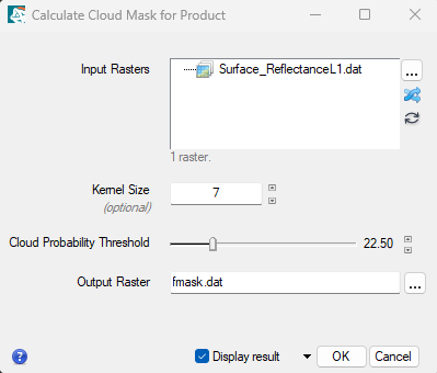
9. When processing is complete, the cloud mask is displayed and added to the Layer Manager. The cloud mask is a binary image where cloud (masked) pixels have values of 0 and non-cloud (non-masked) pixels have values of 1. Visually evaluate the effectiveness of the Fmask process by toggling the layers and/or classes (clouds/ no clouds). Note what features are included in the mask and which are not.

View the Landsat QA Band and Create a Custom Mask

Landsat data products also include Quality Assessment (QA) bands to identify the pixels that exhibit adverse instrument, atmospheric, or surface conditions. This can include clouds, cloud shadows. This information can also be used to generate masks to exclude or isolate certain pixel types from analysis. There are several external tools available to extract information from the QA bands : https://www.usgs.gov/landsat-missions/landsat-collection-2-quality-assessment-bands.

10. Now we will open the Landsat QA band for your selected dataset (Level-1 or Level-2), Select file open and in your Originals folder and select the file "LC09_L1TP_.....QA_PIXEL.tif" Or ""LC09_L2SP_.....QA_PIXEL.tif" and click OK. This is the Landsat Quality Assessment band for the data.
11. Use the cursor value tool to investigate what some of the pixel values are for various features (clouds water etc). You may want to open a new view or toggle between the Landsat surface reflectance layer and the QA band layer for comparison. Make note of some of the QA pixel values associate with clouds, shadows and other features that you might want to mask.
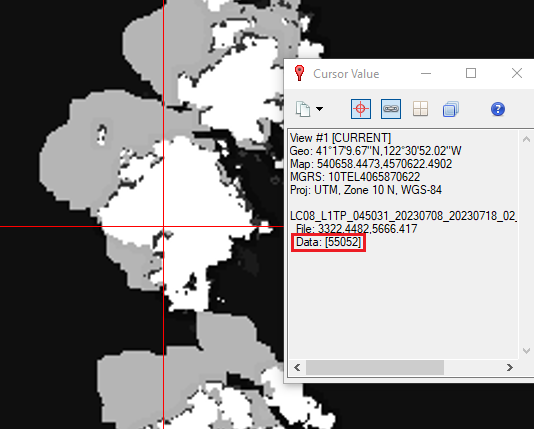
12. Now we will create a ROI (Region of Interest) to use create a mask. Multiple ROIs can be employed to create a mask or you can create a single ROI that includes all features to be masked. Right click on the Surface Reflectance file and select New Region of Interest.
13. You can select specific features using several different methods. Use the threshold option to select certain pixel values in the ROI. Experiment using different bands and the QA bands to try and isolate certain features in the image. For example clouds tend to have relatively high reflectance across the spectrum while water and cloud shadows have low reflectance. Depending on the scene and masking requirements you may want to create multiple separate ROIs for different features. You can also create multiple threshold rules for an ROI.
14. Using one of the above techniques create a mask that masks specific features, note that clouds and no-data areas should be masked in all masks. You will apply this mask when calculating a spectral index of your choice in the next step. Choose one of the following masks to create:
    1. Mask all non-lands areas - ideal for using with spectral vegetation indices like NDVI, NBR etc
    2. Mask all non-water area - ideal for studying water, indices like NDTI, NDCI etc.
    3. Mask all non-snow areas - ideal for studying snow reflectance with indices like NDSI

15. Now we will build the raster mask. From the Toolbox, select Raster Management > Build Raster Mask. The Build Mask Input File dialog appears.

16. Select the input file of Surface Reflectance and click OK. The Mask Definition dialog appears. From the Mask Definition dialog menu bar, select Options, here you can choose to add specific values to mask or ROIs to include in the mask. Under options select the import ROIs option and add the ROI(s) you created in the previous step. If the input file has a data ignore values (no data values), then the dialog opens with these values automatically entered in these fields.
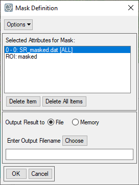
17. Under Options change the mask option to "Selected Areas Off". This will produce a mask where the selected ROI(s) and no data values are masked or "off". Save the file as custommask.dat in the working folder and click OK. Compare the Fmask and your mask results.

Calculate Spectral Index and Apply Mask

ENVI can calculate a variety of different spectral indices. Spectral indices are combinations of spectral reflectance from two or more wavelengths that indicate the relative abundance or characteristics of specific features. ENVI Spectral Indices

18. From the Toolbox, select Band Algebra → Spectral Indices or type "Spectral Indices" in the Toolbox and open the Spectral Index tool. The Spectral Indices dialog appears. Select the final Surface Reflectance data as your Input Data and click Mask button towards the bottom of the window.
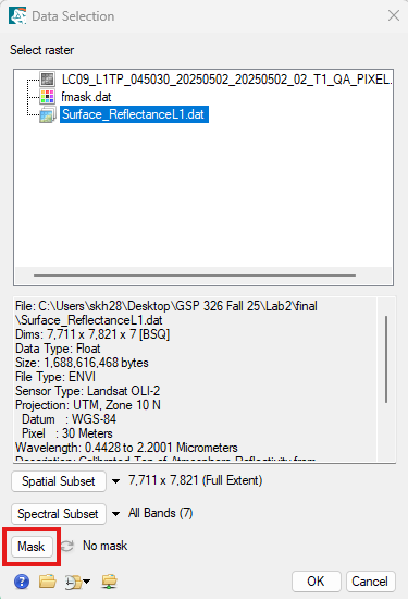
19. In the Mask selection window select the mask from previous steps and click OK.
20. Now you will select the desired Spectral Index from the Spectral Index list. Select a spectral index of your choice, see step 14. Name your output raster appropriately and save it in the finals folder as a .dat file. Click OK and by default the spectral index image should appear in the viewer.
21. After masking, check if a data ignore value is specified. If not, select the Edit ENVI Header tool or view the metadata and click the Edit Metadata. Add the Data Ignore Value Metadata field. Then specify an appropriate data ignore value. This value should not represent any real data values in your image, -9999 or 9999 are commonly used. Save and update the metadata, and you’re good!
22. Now try two different ways to visualize the data. Right click on the "spectral index" layer in the Layer Manager and select "Change Color Table" and select one of the color tables. Applying a Color Table makes it easier to see the differences in spectral indices (or any index) values. Another way to display and investigate data values is using the Raster Color Slice tool. Right click on the layer and select New Raster Color Slice. Select the desired spectral index layer to create a raster color slice with. This will shows you colorized classes that correspond to specified data ranges. You may close or remove the Color Slices when you are done.

Download SRTM Elevation Data in ENVI

23. Now we will download a Digital Elevation Model of the region to use later when creating maps. There is a built in DEM downloader in ENVI that downloads data from the SRTM (see more below).In ENVI, select File > Open World Data > Download Digital Elevation Model from the ENVI menu bar.

    About the Tool and Data
    Use this tool to download Shuttle Radar Topography Mission (SRTM) raster Digital Elevation Model (DEM) data. SRTM raster DEM data is available from https://srtm.csi.cgiar.org/. The SRTM data available through this download option is global, 90 m spatial resolution. The Download SRTM Raster DEM dialog appears. Follow the steps below to define an area of interest, buffer distance, and output coordinate system for the download.

    
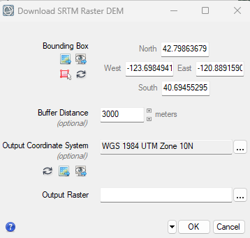
24. Set the Bounding Box as the Surface Reflectance data. This will download a DEM that covers the entire region of the Landsat image. You can also specify other extents manually or using current view. Set the Output Coordinate System to also be the same as the Surface Reflectance data. This means the data will automatically be re-projected to whatever coordinate system you select.
25. Save the output raster as DEM.dat in your finals folder and click OK.
26. After downloading and processing the DEM will appear in the window. It should cover the extent of the Landsat image plus a buffer area surrounding the image. Double check that all of your data (Landsat imagery, Spectral Index and DEM) are all saved in your Final folder.

Visualizing Raster Data in ArcGIS Pro

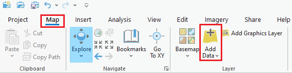
27. Launch ArcGIS Pro and log in using your Humboldt credentials. Open a new blank Map template, call the project Lab 2 Maps and save it to your final folder. A new project and map template are generated. Remove the default basemap layers.
28. Now we will add data to our map. Go to Map tab > Add Data and located the image Surface Reflectance Landsat satellite image from your lab data from the previous lab and open the image (click once to open the color multispectral imagery, double clicking allows you to open individual band). If prompted say yes to Calculating Statistics and Pyramids for the file.
29. There are specific rendering options available for raster files in the Raster Layer tab. Explore the difference Stretch Types and their effect on the imagery. Also try out Resampling Type options to see how they alter the image.
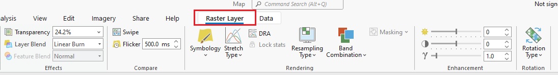
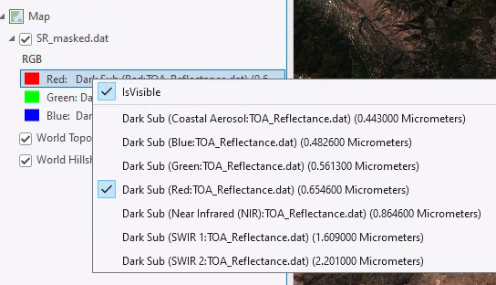
30. You can change the band combinations to any false color composite. Right click on the layer in the table of contents and you can select which band should be displayed in which color (Red, Green, Blue). You can also set and save custom band combinations from the Band Combinations window.
31. There are also a few more image enhancement tools that change the look of imagery. You can adjust the Contrast, Brightness and gamma. You can also adjust the rotation to change from the default of North is up when applicable.

Visualizing Spectral Indices

32. Now add the your spectral index layer and DEM layers that you created in ENVI to your map.
33. Change the symbology of the spectral index layer. Try out different color ramps and symbologies. Try changing the symbology to the classified option and experiment with different colors and classification schemes.
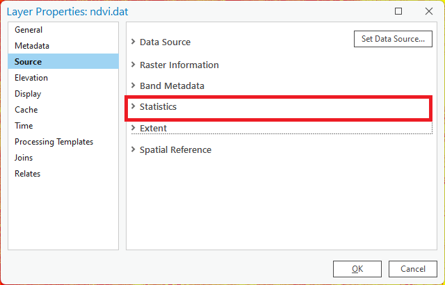
34. Now we will investigate the statistics of the spectral index dataset. Right click on the file and select properties. In the Layer Properties window select the Source tab. This contains information about the raster, including the resolution, coordinate system and summary statistics. Click on statistics and note the mean, min, max and standard deviation of the data.
35. Now we will view a histogram of the spectral index data. Under the Raster Data tab go to Create Chart > Histogram. The Histogram tool appears. Select the spectral index as the number variable.
36. Increase the number of bins, experiment different options. Check the boxes to add the Mean and Standard Deviation to the histogram, then export the graph by selecting Export >Export as a Graphic and saving the image in your finals folder.

Raster Functions

Raster functions are operations that apply processing directly to the pixels of imagery and raster datasets, as opposed to geoprocessing tools, which write out a new raster to disk. Calculations are applied to the pixels of the original data as the raster is displayed, so only pixels that are visible on your screen are processed. These tools are a great way to quickly preview an operation or to create layers for visualization. If you need to save the file or use it in future analyses the geoprocessing tools are more appropriate.

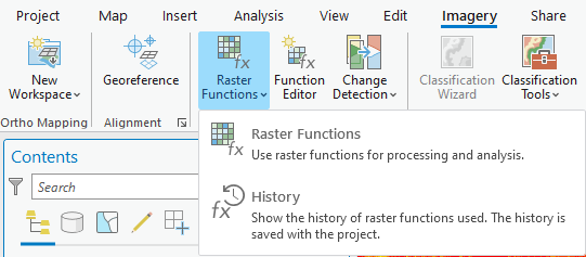
37. Under the Imagery Tab navigate to the Raster Functions button and click on the Raster Functions. This will launch the Raster Functions pane on the side. There are many different functions to choose from.
38. Navigate to the Surface functions in the Raster Functions tool pane. Select the Hillshade option.
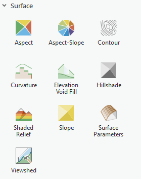
39. Create a hillshade using the DEM as the input file (you can keep all of the default settings).
40. Now create contours, aspect and slope all using the DEM as the input file. Now you have a few topographic layers that can be used to create maps and better visualize your data. If you want to permanently save the layers you created, you will need to export the layer as a standalone file (e.g., TIF) by right-clicking on the layer in the Contents pane and select Data > Export Raster.
41. Rearrange your layers so that the Landsat image is on top of the hillshade (you may choose to leave the contours on or off, your choice). Adjust the settings using the transparency and other enhancements to create a visually appealing satellite image where the topography is slightly visible.

Creating Maps

43. Zoom in on an area of interest to focus on for your map (can be anywhere!). After zooming in go the the Map tab > Bookmarks and click New Bookmark. A bookmark is a navigation shortcut to a position on a map. Name your bookmark.
44. Create a copy of your map by going to the Catalog Pane and right clicking on your map and selecting Duplicate. Paste the map in the Maps folder in the Catalog pane. Repeat the process one more time so you have three maps in your folder. Re-name the maps something like "Landsat", "Spectral index" and "Topographic". You will have three separate maps when you are done. Add the maps to your project by double clicking on them in the Catalog.
45. In each of your maps layer the applicable data layer over the hillshade and adjust to visualization settings. One map should have the satellite imagery as the focus, another with the spectral index results and a final map with the elevation (or other topographic features like slope or aspect) and hillshade and/or contours. All maps should utilize the hillshade to provide topographic relief.
46. Now we will prepare the map layout, we will create one page with all three of our maps and the histogram. From the Insert tab select → New Layout to add a layout to your project. Select a Landscape Letter 8.5" x 11" paper size and press OK. Feel free to adjust the size of the layout as needed.
47. To add a map frame to your layout, click the Map Frame button on the ribbon. From the drop-down, Under the Landsat map select your saved Bookmark as the extent then click on the empty map page. You will now see a rectangle with the default map.
48. Repeat this process to add the remaining two map frames. You should have three map frames on your layout, one with satellite imagery, one with the spectral index and one with topography. Adjust the size of the frames and paper as you see fit. To remove the service credits remove the basemap layers from your map. You may need to switch between the layout and map views for the map to update.
49. Now add the Histogram Chart you made to the layout by going to Insert > Chart Frame and selecting the histogram you created in previous steps.
50. Now add the appropriate cartographic element, including Titles, Labels, Scale bars and North arrow. These can all be found under the “Insert” menu in the Layout View. Also include the data sources and map author.
51. When you are happy with your map export it to a PDF or JPG. Click on the Share tab from the main menu and select “Export Layout”. Select PDF or JPG as the type and make sure the resolution is set at 300dpi and save it in your “Finals" folder.

Turn In - Maps and Histogram

A PDF Layout with:

• Three data frames showing (the same extent and scale ) the satellite imagery, spectral index results and a topographic map of your choosing.
• Spectral index histogram and statistics